Small-Satellite Synthetic Aperture Radar for Continuous Global Biospheric Monitoring: A Review


1
Samsung SDI Co., Ltd. 130 Samsung-ro, Yeongtong-gu, Suwon-si, Gyeonggi-do 16678, Korea
2
Department of Nuclear Engineering, Hangyang University, 222 Wangsimni-ro, Seongdong-gu, Seoul 04763, Korea
3
Department of Aeronautics and Astronautics, Massachusetts Institute of Technology, Cambridge, MA 02139, USA
*
Author to whom correspondence should be addressed.
Remote Sens. 2020, 12(16), 2546; https://doi.org/10.3390/rs12162546
Submission received: 26 June 2020
/
Revised: 23 July 2020
/
Accepted: 2 August 2020
/
Published: 7 August 2020
(This article belongs to the Special Issue Global Biospheric Monitoring with Remote Sensing)
Abstract
:Space-based radar sensors have transformed Earth observation since their first use by Seasat in 1978. Radar instruments are less affected by daylight or weather conditions than optical counterparts, suitable for continually monitoring the global biosphere. The current trends in synthetic aperture radar (SAR) platform design are distinct from traditional approaches in that miniaturized satellites carrying SAR are launched in multiples to form a SAR constellation. A systems engineering perspective is presented in this paper to track the transitioning of space-based SAR platforms from large satellites to small satellites. Technological advances therein are analyzed in terms of subsystem components, standalone satellites, and satellite constellations. The availability of commercial satellite constellations, ground stations, and launch services together enable real-time SAR observations with unprecedented details, which will help reveal the global biomass and their changes owing to anthropogenic drivers. The possible roles of small satellites in global biospheric monitoring and the subsequent research areas are also discussed.
1. Introduction
Space-based radar observation has growing potentials for monitoring the global biospheric diversity subject to anthropogenic drivers at geological scales [1]. The performance of radar is less affected by weather and sunlight conditions than that of optical sensors. Satellites with onboard sensors can provide comprehensive coverage of remote areas or vast regions that may be too costly for unmanned aerial vehicles (UAVs) or ground-based platforms, provided that all platforms provide congruent results via calibrations [2,3,4]. Therefore, it was Seasat, the first satellite dedicated to remote sensing of the Earth’s oceans, that carried the first synthetic aperture radar (SAR) and other radar instruments operable in space. Despite these advantages, miniaturization of radar-carrying satellites was rather slow compared to satellites carrying optical devices due to the lack of commercial-off-the-shelf (COTS) components as well as challenging design requirements for the satellite platform [5,6].
Representative use cases of space-based radar include altimetry, sounding, scatterometry, and so forth in the studies of land, cryosphere, and oceans. Biospheric monitoring is another useful application because radar has high sensitivity in detecting surface changes in a target area and discriminating mobile targets against a background [7]. This paper will consider mainly SAR because of its three-dimensional mapping capability through interferometry. The heritage of Seasat has influenced many of later SAR missions for decades, as listed in Table 1 [8,9,10,11,12,13]; for instance, Shuttle Image Radar (SIR) missions used spare parts of the previous Seasat mission onboard Space Shuttles to test SAR image applications in land use, geology, hydrology, and forestry [14,15]. European Remote-Sensing Satellite (ERS) could obtain radar data in polar regions thanks to its polar orbit. Two different operational modes were available for SAR of ERS, the imaging mode for high resolution (10m) and the wave mode with 30m resolution for vector measurement of ocean waves. Figure 1 describes the acquisition of imagelets during the wave mode, which may be subdivided into the On-Ground Range Compression (OGRC, 5 km × 5 km) mode and the Onboard Range Compression (OBRC, 5 km × 9.6–12 km) mode [16]. The imaging mode, not shown in Figure 1, is identical to the wave mode except that the entire 100 km wide strip is scanned for high-resolution imagery without any movement profile information. This resolution-swath tradeoff is also shown in Advanced Land Observing Satellite (ALOS) whose ScanSAR mode has a coarse 100m resolution but 250–350 km wide swath. This is 3 to 5 times wider than conventional SAR images and is especially useful for monitoring sea ice and rain forest extent with expansive areas of interest [13].
An important application of SAR is interferometric synthetic aperture radar (InSAR), which was first attempted by time-series analysis of Seasat data. The phase difference in two or more SAR images is measured to yield centimeter- or millimeter-level surface changes over large areas (squares of km) at meter-level resolutions, making InSAR ideal for monitoring surface deformations of Earth [17]. The SAR images capturing the same scene may be acquired at two different times and/or at two slightly different locations. The technique has matured since ERS in the 1990s when the stabilization of satellite orbits allowed for exploiting repeat-ground tracks to visit target areas on a regular basis [18]. Japanese Earth Resources Satellite 1 (JERS-1) also demonstrated two-pass (repeat-pass) cross-track interferometry, meaning that different radar images are obtained from different orbits at different moments [19]. It was the US-Germany joint mission in 2000, called Shuttle Radar Topography Mission (SRTM), which performed single-pass interferometry using one radar antenna onboard a Space Shuttle and another mounted on the end of 60-m mast connected to it [20]. As its name suggests, SRTM was a continuation of the SIR mission in 1994 with a two-antenna configuration. This two-antenna SAR concept is further being developed by German twin-satellite missions as technologies for close-formation flight have become reliable [21]. These missions have new observation modes such as along-track InSAR and SAR polarimetry [22].
Traditional research interests utilizing SAR data focused on geosphere, hydrosphere, and cryosphere among different realms (“-spheres”) of Earth science [23,24,25]. Note that the atmosphere is not included in Table 2 because the purpose of radar observation is to minimize the weather influence on its data; ocean wind, for example, is covered by hydrosphere in the context of its surface interactions. Biospheric monitoring herein involves efforts to apply SAR data to agriculture, forestry, and the studies of grasslands and wetlands [26,27]. When it comes to the interactions between the biosphere and the anthroposphere, SAR data could benefit urban management, resource exploration, biomass monitoring, vulnerability studies (e.g., diseases) to name a few as will be seen in Section 4 [28,29,30,31,32]. The vulnerability studies may also involve interactions between anthroposphere and other realms such as geological events leading to disasters, which again affect biosphere [33]. This trend testifies the newly increasing importance of biospheric monitoring for the already mature field of SAR-based Earth remote sensing.
Hitherto, spaceborne SAR instruments have been flown onboard monolithic satellites whose mass is a few tons. On the other side of monolith satellites is the category of small satellites. A small satellite (“Smallsat”) weighs less than 500 kg and may be called by other names according to its mass, as listed in Figure 2 [34,35]. Small satellites have become an active area of research as the CubeSat platform was standardized by California Polytechnic State University and Stanford University in 1999 [36]. The CubeSat platform consists of multiple units (“U” s), which is a 10 × 10 × 10 cm cubit volume and is therefore also called “U-class” spacecraft. In terms of mass, a 1 to 3U CubeSat weighs between 1~4 kg, falling into the nanosatellite regime in Figure 2 [37]. Although some of the optical sensors have reached the extent of miniaturization as well as commercialization to fit into a 3U class (e.g., Planet) that has a size of a shoebox, most of the advanced sensors featuring multiple bandwidths require larger volumes, i.e., 6U or more [38,39]. Due to its lower operational frequency (longer wavelength), a radar antenna should be larger than satellite payloads that operate in visible, infrared, or microwave spectrums. The radar system also requires higher power throughputs than optical payloads because they must transmit electromagnetic pulses first to the ground before receiving the backscattered echoes [8,40]. Despite these challenges and constraints, there are several mission plans and startup initiatives for Earth observation missions with SAR-equipped small satellites, which are driven by the aforementioned scientific needs as well as performance-cost advantages of Smallsat constellations [41,42]. Biospheric monitoring is more explicitly manifested as a scientific objective of large SAR satellites, and the same is expected in Smallsat constellations as well [26,43,44].
The organization of this paper is as follows: Section 2 briefly introduces SAR design principles. Section 3 investigates current or planned small satellite missions, paying extra attention to their operational details and constellation design if applicable. In addition to minisatellite- and microsatellite-SAR, some larger SAR spacecraft and Cubesat-level non-SAR nanosatellites are also considered. Section 4 concludes with potential use cases of small-satellite SAR in global biospheric monitoring as an extension of larger SAR missions.
2. Design Principles of Synthetic Aperture Radar
The underlying physics is identical between large-satellite SAR and small-satellite SAR in their design process, but the optimization goals might be different. Design principles of Smallsat SAR are unconventional in that minimizing the antenna sizes and the number of observation modes has priority over improving the ground resolution, whose trend is prominent under the launch mass of 200 kg [45]. In general, the best possible ground resolution for stripmap SAR in the along-track (azimuthal) dimension is given by:
where La is the along-track (azimuthal) physical length of the SAR antenna, which is illustrated in Figure 3 (left). To avoid ambiguity and maximize the swath, the minimum antenna area that is the product of La and the across-track (cross-track) width Wa should be:
where V is the satellite speed (~7 km/s), λ is the radar wavelength, c is the speed of light, Rm is the range to the middle of the swath, and η is the look angle. The corresponding swath is
under the condition that the ground swath must be wider than the antenna footprint on the ground at the minimum pulse repetition frequency (PRF) equal to 2V/L or the Doppler bandwidth [46]. From the linear relation between the ground swath and the antenna size, it is possible to reduce the antenna length without sacrificing the ground resolution by accepting a smaller swath, or vice versa. The antenna width may also be reduced with a smaller noise bandwidth. The following expression shows, however, that reducing the antenna width (Wa) has squaring impacts that must be absorbed by the noise bandwidth (Bn), the transmit pulse duration (τp), the peak transmission power (Pt), or the antenna length in order to keep the signal-to-noise ratio (SNR) constant:
The ground-range resolution is dependent on the chirp bandwidth as well as the incidence angle:
where by better ground-range resolution would increase the bandwidth and thus require a higher transmitter power per Equation (4). Unlike 2-D optical images, this altimetry capability of SAR leads to numerous 3-D applications, which is why the ground-range resolution is an important performance metric; the design specifications of an optical satellite only mention ground sample distance (GSD) whereas SAR satellites are usually specified by both azimuthal resolution and ground-range resolution as listed in Table 1. Figure 3 (right) describes the multi-parametric dependence of ground-range resolution on look angle and bandwidth.
The data rate should also be carefully chosen to maximize on-time of SAR and the transferrable data volume, under the ground station constraints, in addition to the relationship among the antenna size, the orbit geometry, the SNR, and the power requirement. Small satellites usually minimize the number of observation modes and the number of channels to cope with their inherent design constraints. While smaller and more efficient commercial-off-the-shelf (COTS) parts are becoming available with respect to communications and power electronics, even more innovative technologies such as inter-satellite links (e.g., optical laser communications) or wireless power transfers may be envisioned.
3. Synthetic Aperture Radar Satellite Missions
This section surveys spaceborne SAR missions flown already or being planned. First, earlier SAR missions featuring satellite constellations or formation flight are covered in Section 3.1.
3.1. Medium/Large Satellite Constellations
SAR missions in Table 1 have satellite launch mass greater than 500 kg and do not technically fall into the small satellite category. Either medium (500 kg to 1 ton) or large (>1 ton), these satellites were designed following rather conventional principles, less affected by design constraints in mass and volume than small satellites. Nonetheless, deployment and operation details of missions in Table 1 still provide useful guidelines. For example, SAR-Lupe is a 5-satellite system and Cosmo-SkyMed is a 4-satellite system, being the largest and the second-largest (homogeneous) constellations launched so far. Future missions with larger numbers of small satellites would require efficient strategies for constellation design and deployment, for which SAR-Lupe and Cosmo-SkyMed could be good references. TanDEM-X demonstrates various formation flight technologies with two satellites flying close to each other in space, and HJ-1C is an interesting example of a heterogeneous constellation of SAR platforms and optical platforms.
3.1.1. SAR-Lupe
SAR-Lupe is Germany’s first military satellite system for global surveillance, delivering radar images for the German Armed Forces for at least ten years since its launch. The spacecraft design by the OHB-System AG utilized a parabolic reflector antenna instead of active beam-steering antennas, which led to major savings in the cost of instrument development [47,48]. However, the size of a reflector antenna (3.3 m × 2.7 m) poses a major volume constraint during satellite stowage and launch phases as shown in Figure 4, necessitating a dedicated launch for each satellite. The five identical SAR satellites were launched between 2006 and 2008, with individual launches separated by 4 to 8 months [49]. The five satellites are distributed in three orbital planes, marked with plane numbers and corresponding satellites in Figure 4 (right). Orbital planes 1 and 2 are separated by 64° in longitude, and orbital planes 2 and 3 are separated by 65°. Satellite-pairs in orbital planes 1 and 3 have phase angles differing by 69°. Together with a near-polar inclination (98.2°), this satellite arrangement provides the SAR-Lupe constellation with both global coverage and short response time.
Observation of SAR-Lupe is made in the X band with a frequency of 9.65 GHz and a wavelength of 3.1 cm, capable of change detection based on SAR interferometry [50]. The stripmap (60 km × 8 km) observation of SAR-Lupe provides nadir-looking scenes, whereas the spotlight (5.5 km × 5.5 km) scenes require the orienting of a spacecraft towards a target area to increase integration time for 0.5 m resolution. When the image acquisition is complete, the spacecraft returns to its standby mode for recharging two 66 Ah lithium-ion batteries with solar panels. Amongst L, S, C, and X bands listed in Figure 5 used for radar sensors, the X band requires the smallest antenna size, which enabled the adoption of a parabolic antenna whose size would be unacceptable in other spectral bands [51]. It also led to a compact design of power systems such as solar arrays providing 550 W at the end of life (EOL), an order of magnitude smaller than the 7 kW power generation (EOL) by ALOS in Table 1. When it comes to onboard batteries, ALOS used nickel-cadmium batteries and SAR-Lupe used lithium-ion for the first time in SAR satellites. Although lithium-ion batteries do not have a “memory effect” suffered by nickel-cadmium batteries, they only became available after more lenient electric-power requirements owing to their higher costs. After all, SAR-Lupe is an interesting example featuring efficient onboard power management at a spacecraft level and a constellation architecture with multiple orbital planes at a higher level, both of which inspired later SAR constellations with small satellites.
3.1.2. Cosmo-SkyMed
COSMO-SkyMed is the acronym for Constellation of Small Satellites for Mediterranean Basin Observation, conceived by the Italian Space Agency. Funded by the Italian Ministry of Research and the Italian Ministry of Defense, the satellite system has dual-use (civilian and military) applications ranging from reconnaissance and risk management to the monitoring of biospheres such as marine/coastal environments, agriculture, and forestry. Because the launch dates of the first satellite (June 2007) and the last satellite (November 2010) are more than three years apart, the constellation size grew rather gradually, operating with intermediate configurations. In each phase, all satellites are in the same orbital plane; the inter-satellite angle decreased from 180° in two-satellite configuration to 90° in a four-satellite configuration in Figure 6. The coverage performance during each stage is listed in Table 3 and Table 4; the mean revisit time of 3 to 6 h at the full-blown state is still longer than three-plane SAR-Lupe whose revisit time is expected to be about an hour [52,53].
However, the all-in-one-plane architecture of COSMO-SkyMed enables easy transition of its orbital configuration from the nominal mode to several interferometric modes, namely “tandem” and “tandem-like (one-day interferometry)” [54]. First, in tandem interferometry, two satellites are separated in two orbit planes slightly differing in the ascending nodes by 0.08°, denoted as AN (blue) in Figure 6, to guarantee exactly overlapping ground tracks. If the satellites are in a single orbit, they will have slightly different ground tracks due to orbital regression, which is called J2 (Earth’s oblateness) effects [55]. The phasing of the two satellites is also adjusted such that the resulting leader-follower pair achieves identical incidence angles. In other words, the two satellites acquire imagery of the same scenes with the same geometry, with a delay of 20 s. Second, in the tandem-like configuration, two satellites stay on the same orbit plane at a distance of 67.5°. This specific angle is used instead of 90° for the tandem-like configuration to achieve “one-day interferometry” with 237/16 repeat cycles; a satellite in this orbit completes 14 and 13/16 revolutions after 16 days (denominator), and the remaining 3/16 revolution to complete an integer number corresponds to 67.5° (=3/16 × 360). The two satellites with this phase spacing visit the same ground target with an exact 1-day interval, as illustrated by COSMO-2 and COSMO-3 in Figure 7 (right). The orbit is a sun-synchronous orbit with an inclination of 97.86°, a nominal altitude of 620 km, and the local time of the ascending node (LTAN) at 6:00 (dawn/dust orbit).
The radar transmitter and receiver of each COSMO satellite operate through an electrically steerable multi-beam [56]. This active sensing scheme necessitates a COSMO satellite to manage and store its electrical power more efficiently than other passive SAR systems (e.g., SAR-Lupe). The nominal capacity of a COSMO satellite is 336 Ah, nearly three times larger than that of a SAR-Lupe satellite. The battery cells constituting a COSMO satellite are much smaller in size, however, with 18-mm-wide, 650-mm-long cylindrical footprint depicted in Figure 8 (left). A total of 2016 lithium-ion cylindrical cells are connected in a 9s224p configuration, meaning that 9 cells are first connected in series and then 224 such series-strings, distributed across eight modules in Figure 8 (right), are connected in parallel [57,58]. This configuration provides a maximum current of 650 A (460 A for the 10-s maximum duration) in Spotlight mode and 450 A (330 A for the 10-min maximum duration) in Stripmap mode. The power consumption of a SAR payload in the two modes is 13 kW and 7 kW, respectively. The power subsystem supports a fully polarimetric SAR (PolSAR) where only one linear polarization is received at each interrogation [59].
Both SAR-Lupe and COSMO-SkyMed constellations reserve the capability of their satellites to reconfigure their orbits. The resulting launch mass or each satellite was a ton or more, however, electric propulsion seems to be an alternative of chemical propulsion for small satellites to achieve miniaturization, as will be discussed later. Still, medium-to-large satellites will continue to provide responsive access to observation targets, complementing small-satellite constellations’ wide coverage [52,53]. The COSMO-SkyMed mission demonstrated another way of cost reduction using commercial cylindrical lithium-ion batteries for power storage, which can be applied to small satellites as well.
3.1.3. TanDEM-X
The TanDEM-X (TDX, 2007) mission is an extension of the TerraSAR-X (TSX, 2010) mission flying two identical satellites in a close formation to achieve a highly flexible SAR constellation. Following the previous mission name (TerraSAR-X), TanDEM-X means “TerraSAR-X add-on for Digital Elevation Measurement,” both of which were implemented through a Public-Private-Partnership of the German Aerospace center (DLR) and European Aeronautic Defense and Space (EADS) Company Astrium (now Airbus Defense and Space). The SAR payload of both TDX and TSX has flight heritage dating back to Shuttle missions such as SIR-X and SRTM, which tested the single-pass SAR interferometry (InSAR) in the X band [60]. The primary objective of the mission is digital elevation model (DEM) generation, for which bistatic processing is employed [61]; both spacecraft, less than 2 km apart as represented in Figure 9 (left), orient their SAR instruments to a common target, which provides different viewing angles [62]. Both spacecraft simultaneously receive echoes of signals transmitted by one of them, which minimizes temporal decorrelation. The resultant single-pass interferometry does not suffer accuracy loss, which would affect repeat-pass (multi-pass) interferometry with a single satellite. An example of bistatic InSAR is the TanDEM-X Forest/Non-Forest Map in which the global raw data set with 50 m × 50 m ground independent pixels were used to classify forest and non-forest areas (urban settlements or freshwater), as shown in Figure 10 [63]. The second interferometric mode is the pursuit monostatic mode, whose Tx/Rx operations are decoupled in two satellites as shown in Figure 9 (right). The amount of temporal decorrelation therein is still small compared to the repeat-pass counterpart. In addition to the aforementioned multistatic (bistatic or monostatic) baseline, the TDX mission concept demonstrated the along-track interferometry (ATI) with four inter- or intra-satellite phase centers. The ATI technique can be used to resolve the velocity of ocean currents, ice drift, and other on-ground objects (e.g., transportation traffic) [64,65,66].
The TSX spacecraft retains its sun-synchronous dawn-dusk orbit (LTAN = 18:00) with a 515 km altitude and a revisit period of 11 days with 167 orbits, or 15 and 2/11 revolutions per day. The TDX orbit uses eccentricity-inclination separation with respect to the TSX orbit, through which the two spacecraft leave a helix-shaped trajectory relative to a virtual reference in between. The procedures for eccentricity-inclination separation and the relative trajectory are depicted in Figure 11. First, the ascending node of the TDX orbit plane is shifted by a small offset angle to provide horizontal distancing with maximum distance at equator crossings, and the subsequent eccentricity offset provides vertical (radial) distancing maximized at the poles. Small changes in the argument of perigee may also be made to increase inter-satellite distance in medium latitude regions. This kind of orbit and its building procedure have been proposed for consistent separation distance, which in turn reduces collision hazards evenly along the orbit [67,68].
The remote sensing data obtained from TSX/TDX missions have been widely shared with and studied by the scientific community including the TanDEM-X Forest/Non-Forest Map available free of charge online [25,69]. Differencing digital elevation models taken at different moments in time can be applied to monitor climate change, for example, in polar regions. For the first time, pan-Arctic InSAR is made possible with TDX and was applied to observations of a thaw slump in the Mackenzie River Delta, Canada whose aerial photo is provided in Figure 12A [70,71]. The swamp whose DEM was taken in 2015, shown in Figure 12B, has grown in size compared to 2011, which is represented by negative height changes (depression) in Figure 12C. In addition to this differential InSAR (DInSAR), polarimetric InSAR (Pol-InSAR) by TSX/TDX enables multi-temporal, detailed vertical mapping of croplands and wetlands, which is further discussed in Section 4 [72,73,74]. Lastly, 3D SAR images can be constructed from multitudes of 2D SAR images taken at slightly different angles, which reduces ambiguity in pixels with the identical range from satellite but different terrain elevations. This technique of SAR tomography is being applied to deformation analysis of rigid bodies including glaciers and urban infrastructure, as shown in Figure 13 [70,75].
The nominal design life of TSX and TDX spacecraft has ended in 2012 and 2015, but as of March 2016, the two spacecraft were still operational with similar amounts of residual propellant (TSX: 55%, TDX: 56%) [76]. The fact that calibration of radar instruments did not show any signs of degradation implies the future possibility of extending the lifetime of a medium-sized SAR spacecraft if desired; on-orbit servicing was first demonstrated to refuel a communications satellite in 2020 [77]. The residual capacity of onboard lithium-ion batteries is a function of time, gauging 74% and 82% of the initial 108 Ah for TSX and TDX, respectively. The available spacecraft power has decreased from the peak power of 1.8 kW at the beginning of life (BOL) to the orbital average of 800 watts at the end of life (EOL), which could affect the capability of radar radiation and data communications. The design life of smaller SAR satellites is significantly shorter (<3 years) where the degraded performance should be taken into account for constellation deployment and maintenance because refueling them would not be economical [52,78].
3.1.4. HJ-1C
Being China’s first civilian radar satellite, HJ-1C is part of the HJ-1 (Environment-1) constellation implemented by the National Committee for Disaster Reduction and State Environmental Protection Administration (NDRCC/SEPA) [79]. HJ-1A and HJ-1B are optical satellites with a hyperspectral camera and an infrared camera, respectively; they were launched together in 2018 and placed into a circular Sun-synchronous orbit with a 650 km altitude, 4-day repeating (recursive) ground tracks, and an angular position difference of 180°. On the other hand, HJ-1C has a launch mass of 890 kg, nearly twice as heavy as the other optical satellites (470 kg), and was launched into a different Sun-synchronous circular orbit with a 500 km altitude and 31-day repeating cycles. HJ-1C has a dawn-dusk orbit, meaning that its LTDN (Local Time on Descending Node) is 06:00 h, which is also different from 10:45 h of the other satellite. The three satellites are heterogeneous, as the “2 + 1 constellation” notation suggests, but share common mission goals of environmental protection and disaster monitoring. Examples of disaster monitoring include flood, drought, typhoons, earthquakes, grassland or forest fires, and oil spills [80]. The flexibility of HJ-1A to vary its orbit-repeating period between 4 and 31 days suggests synchronized interoperability with HJ-1C, which has a 31-day repeat cycle. The S-band SAR was developed with the assistance of Russia, jointly from NPO Mashinostroyenia (rocket design bureau) and Vega Radio Engineering Corporation. The radar powered by two 40 Ah batteries experienced limited functionality due to antenna damage prior to decommissioning [81]. The impacts of such unit malfunctions would be confined in a mission utilizing swarms of small SAR satellites where a unit may be commissioned or decommissioned flexibly.
3.2. Minisatellites
Alike medium/large satellites, existing SAR minisatellites have been launched one-at-a-time despite their volume and mass footprints reduced from medium/large satellites. Actually, minisatellites were just at the verge of enabling a multiple satellite launch onboard a single launch vehicle, which was realized in smaller SAR satellites later.
3.2.1. NovaSAR-1 (400 kg)
Developed by Surrey Satellite Technology Ltd. (SSTL) and Astrium UK, NovaSAR-1 is one of the first low-cost SAR satellites that are both small and commercial [82]. Potential use cases of NovaSAR-1 imagery include tropical forest protection, disaster monitoring, and maritime services to detect ships, icebergs, and oil spills [83,84]. The observation modes of NovaSAR-1 and their characteristics are summarized in Table 5 [85]. The originally envisioned constellation had three “NovaSAR-S” satellites operating in the S band. Only one satellite, named NovaSAR-S 1 or NovaSAR-1, has been in orbit since 2018. The operational parameters and the revisit performance for each observation mode are provided in Table 5. The expected constellation performance shows that the effect of decreasing average revisit time is around a factor of 3; the effect of decreasing maximum revisit time is larger, meaning that week-long revisits are prevented and global monitoring becomes more continuous. The baseline modes in Table 5 use HH or VV polarization, but the payload of NovaSAR can be configured to operate with dual polarization (any 2 from HH, VV, HV, or VH), tri-polarization (any 3 from HH, VV, HV, or VH), or fully-quad polarization (HH, VV, HV, and VH) as well.
As shown in Figure 12A, NovaSAR-1 has a 3 m × 1 m microstrip patch array antenna with 18 elements operating at 3.1–3.3 GHz in center frequency. This S band is located between the L band and the C band but has been seldom utilized since USSR’s Almaz-1 program whose operations terminated in 1992 [9]. An S-band system has operating wavelengths closest to existing C-band systems in particular, suggesting similarly diverse applications already served by C-band systems. While HJ-1C is another example of exploiting S-band frequencies, NovaSAR-1 concentrated on reducing the satellite mass by employing COTS hardware. In lieu of traveling-wave tube amplifiers that are both bulky and high-voltage, NovaSAR-1 used allium nitride (GaN) solid-state power amplifiers. The radio frequency peak power of NovaSAR-1 is a 1.8 kW, 10% to 15% of a Cosmo-SkyMed satellite, where the power subsystem mass was reduced by limiting the duration of each SAR operation to 2 min per orbit. Although much shorter than the 10-min continuous operation of a COSMO satellite, the duration is still sufficient to cover a nation-state in most cases. Through these miniaturization measures, the interior of NovaSAR-1 still has unoccupied space, as shown in the middle of Figure 14 (left), with further miniaturizablity for an active beam-steering SAR satellite. Figure 14 (right) shows a SAR image capturing the vicinity of the Suez Canal at 30 m resolution. The Commonwealth Scientific and Industrial Research Organisation (CSIRO) of Australia has purchased 10% share of NovaSAR’s acquisition time to improve flood forecasting systems [86]. Similar to larger SAR missions such as COSMO-SkyMed and TSX/TDX, NovaSAR adopted Sun-synchronous orbits with LTAN at 10:30 am. This Sun synchronism is a common practice in designing Earth-observing optical satellites because of advantages in power generation and thermal controls, which is the same for SAR satellites. From a remote sensing perspective, temperature or moisture conditions, as well as solar illumination, tend to be consistent in ground targets if observed at the same time of the day.
Although a Dnepr rocket may launch up to 3 NovaSAR at once theoretically, multi-satellite launches have not been realized for NovaSAR and other minisatellites; further miniaturization was necessary, which was achieved by microsatellites introduced in the next section. The notable milestone of NovaSAR, however, is that SSTL became the first satellite manufacturer with a full Earth-observation line-up covering radar instruments as well as infrared and visible-wavelength payloads (e.g., Disaster Monitoring Constellation in 2002). Continuing its successful contracts of optical satellites with several national governments, SSTL was able to commercialize NovaSAR’s product with Australia and the Philippines, heralding the advent of a global SAR data market [87].
3.2.2. TECSAR (260 kg)
TECSAR, also transcribed as TechSAR, is the first Israeli SAR satellite designed and developed by Israel Aerospace Industries Ltd. (IAI) for technology demonstration of Israeli Ministry of Defense. TECSAR-1, also called Ofeq-8, was launched in 2008 onto a 403 km × 581 km orbit with 41° inclination whereas TECSAR-2, or Ofeq-10, was launched in 2014 onto a 384 km × 609 km orbit with 140.95° inclination [88]. Out of the satellite mass of 260 kg, the SAR payload accounts for 100 kg with 1.6 kW peak power, which is powered by a 45 Ah lithium-ion battery with solar panels capable of generating 850 W of power [89]. This level of miniaturization has been realized by adopting a deployable, umbrella-shaped parabolic antenna. The reflector-based parabolic antenna of TECSAR distinguishes itself from active patch arrays of TerraSAR-X and Cosmo-SkyMed constellations [90,91,92]. The paraboloid reflector consists of skeleton ribs and knitted mesh, the latter of which weighs less than 0.5 kg in mass. At the center of the paraboloid is a rigid dish made of carbon fiber reinforced plastic (CFRP) to combine its advantage in surface homogeneity with the lightweight of knitted mesh in Figure 15 (left) [93]. Among the observation modes of TECSAR, the wide-coverage ScanSAR mode achieves the largest swath up to 100 km with a resolution between 8 m and 20 m. The stripmap mode, mosaic mode, and spotlight mode allocate observation time to a band area, several points, and a single spot, respectively. The resulting resolution decreases from 3 m to 1.8 m and 1 m.
3.2.3. SmallSat InSAR (180 kg)
SmallSat InSAR is a design concept by Jet Propulsion Laboratory (JPL) to demonstrate the technical feasibility and economic viability of a small-satellite SAR constellation [46]. Its design principles were already explained in Section 2, whose volume and mass constraints are derived from the standards of an EELV Secondary Payload Adapter (“ESPA” or “ESPA ring”), which utilizes the unused payload margins of Evolved Expendable Launch Vehicles (EELVs) of the US Department of Defense [94]. Multiple types of ESPA rings and their combinations will provide small satellites with affordable rideshare (or piggy-back) launch opportunities depicted in Figure 16 [95]. Although an ESPA and an ESPA “grande” may allow the maximum spacecraft mass of 320 kg and 450 kg in 6-slot and 4-slot configurations, respectively, SmallSat InSAR aimed to drive the spacecraft mass below 200 kg accommodatable by all six slots of an ESPA ring at the same time. By limiting the spacecraft mass and size (1.0 m × 0.7 m × 0.6 m), shown in Figure 16 (right), multiple SAR satellites can be launched simultaneously for rapid constellation deployment. SmallSat InSAR considered deploying a total of 12 small SAR satellites with two ESPA launches, but its launch schedule is unknown. The peak transmit power of the satellite is designed to be 1 kW.
SmallSat InSAR is often compared with the NASA-ISRO Synthetic Aperture Radar (NISAR) Mission in terms of scientific scopes, mass, and cost. The NISAR mission scheduled for launch in 2021 has multiple purposes of measuring land surface motions and ecosystem disturbances. These objectives can be translated into use scenarios specific to India such as monitoring agricultural biomass, Himalayan glaciers, and coastal environments [96]. The main objective of SmallSat InSAR is to map Earth’s surface deformation with sub-millimeter-per-year precision via daily visits supported by a twelve-satellite constellation. A rough estimate of the total system cost is 1 to 1.5 times the cost of a single-spacecraft NISAR mission. The JPL team’s work dating back to 1999 is based on a systems-engineering philosophy briefly described in Section 2 [45]. The idea of systemizing the design process of SAR satellites and relaxing their design goal for miniaturization was referred to by designers of RADARSAT, TSX/TDX, and Micro XSAR to name a few [97,98,99,100].
3.2.4. Micro XSAR (135 kg)
JAXA/ISAS, University of Tokyo, and Keio University are working on the 100 kg class X-band SAR project whose proto-flight model (PFM) was completed in 2019 and is currently ready for launch [101]. A novel signal processing scheme as well as an efficient waveguide feeder design, with an increased chirp bandwidth of 300 MHz, is capable of providing 1-m resolution at nadir off-set angle of 30° [102,103,104]. Figure 17 (left) illustrates the concept of operations where active or wide-area sensing is made during the day and passive Earth-oriented sensing is made at night. Figure 17 (right) shows possible daytime observation modes, which include underground mapping.
To supply SAR power more than 1.3 kW for several minutes, during the daytime, the solar cells of Micro XSAR charge their lithium-ion battery whose discharge specification is rated at 3 C or the speed of depleting the whole battery in 1/3 h [105]. The estimated battery energy is 400 Wh and the ampere-hour capacity is expected to be similar to or less than TECSAR whose design specifications are summarized in Table 6. Amongst the other satellites in Table 6, Radar In a CubeSat (RaInCube) provides the lower capacity bound of about 10 Ah (similar to an electric scooter) for smaller SAR satellites discussed in the next subsection [106,107,108]. Further advances in power source densities could bring both the cost and footprints down to intensify the advantages of small SAR satellite systems.
3.3. Microsatellites
Sub-100 kg microsatellites are currently the lightest small-satellite class in which SAR has been implemented. Many of these SAR satellites are being developed by start-up companies for commercial purposes and feature rapid design iterations between generations.
3.3.1. ICEYE-X1/X2 (85 kg)
Developed by ICEYE in Finland and launched in 2018, ICEYE-X1 is known as the first SAR in microsatellite class with a design mass of 70 kg as well as the country’s first commercial satellite [109]. In its launch configuration, ICEYE-X1 has a size of 0.7 m (H) × 0.6 m (W) × 0.4 m (D); its X-band antenna has a length of 3.25 m when deployed [110,111]. With 2 to 3 years of designed life, ICEYE-X1 has a similar shape as the Micro XSAR proto-flight model or the SmallSat InSAR concept. Compared to this proof-of-concept version, ICEYE-X2 features increased form factors (0.8 m × 0.8 m × 0.6 m before deployment, 85 kg) to improve the SAR performance, as shown in Figure 18. The RF peak power of ICEYE-X2 is 4 kW, more than twice the ICEYE-X1 capacity, and its SAR imagery resolution also improved from 10 m to a sub-meter level [112]. The fast design iteration can be seen from the launch dates of the two satellites, January 2018 and December 2018, separated by less than a year. The follow-on satellites, ICEYE-X4 and ICEYE-X5, have identical design specifications as ICEYE-X2 and have been launched together in July 2019, which is probably the first case of launching multiple SAR satellites simultaneously. The ICEYE-X3, also called Harbinger, is a military-purpose variant featuring field-effect electric propulsion and high-rate laser communications capabilities whose payload operations demand 3 kW peak power. Harbinger is no longer classified as a microsatellite because its launch mass is 150 kg falling into the minisatellite class. All ICEYE spacecraft except X3 use Sun-synchronous orbits with inclination values of 97.56° or 97.77°; ICEYE-X3 instead uses an inclined orbit with 40.0° for increased visit frequencies in mid- to low-latitude regions [113]. The fully-blown constellation, with a total of 18 ICEYE satellites launched by 2021, will provide an average of 3-h revisit interval around the globe to observe sea ice movements, marine oil spills, and illegal fishing vessels. In addition to its fast design iteration, the fact that ICEYE is the first Finnish commercial satellite exemplifies a strategy of jumpstarting the SAR satellite development, instead of optical/infrared observation satellites, for Earth remote sensing and its data commercialization.
3.3.2. MicroSAR (65 kg)
The MicroSAR system is a proposal by Kongsberg Satellite Services and Space Norway, tailored for maritime monitoring. It is equipped with a C-band 800 W radar transmitter and an onboard automatic identification system (AIS) for vessel tracking [114]. The launch mass of MicroSAR is 65 kg including a 3.8 m × 1.8 deployable reflector illustrated in Figure 19 (left). Figure 19 (right) provides a pictorial description of expected revisit times achieved by eight satellites in two orbit planes in the arctic region. Low-latency tasking and data delivery are possible via a network of twenty ground stations adapted for small satellites across continents and oceans including the Arctic Circle (Svalbard) and Antarctica (Troll Station). Although any MicroSAR satellite has not been launched yet, it represents an example of prioritizing the ground station infrastructures, which have been jointly utilized by Cosmo-SkyMe and NovaSAR. As the demand for SAR data increase and small satellites play a bigger role therein, its market will be segmented into launch services (e.g., Electron rocket), ground stations (e.g., KSAT), data analytics (5. Discussion), and so forth dedicated to small satellites and/or spaceborne SAR.
3.3.3. Capella X-SAR (48 kg)
This SAR constellation, developed by Capella Space, will have 36 satellites by 2023, 6 of which are already in orbit [115]. The first satellite, Capella 1 or Denali, has a launch mass of less than 50 kg with an origami-like antenna shown in Figure 20 (left). The second satellite, Capella 2 or Sequoia, is about twice as large as the predecessor, accommodates a 600 W transmitter and a mesh-based 8 m2 reflector that is shown in Figure 20 (right) to achieve sub-meter ground resolution [116]. Following the launch of Capella 1 in December 2018 and Capella 2 in March 2020, three satellites (Capella 3, 4, 5) will be launched with further design improvements, constituting a “Whitney sub-constellation. Another satellite called Capella X was launched into an inclined orbit with 45° inclination in May 2020. The Whitney sub-constellation and others will constitute the “Capella 36” constellation, and the coverage performance of possible configurations in between is summarized in Table 7. Capella Space is using the satellite ground station service provided by Amazon Web Services (AWS) for the rapid delivery of satellite data to its customers [117].
3.4. Nanosatellites
Due to extreme sizing constraints, nanosatellites use the Ku-band or higher microwave frequencies (~100 GHz) that are increasingly sensitive to precipitation. The sensitivity of resonance bands (e.g., 60 GHz and 118 GHz for oxygen) to precipitation and altitude makes radar sounders that operate at these frequencies with short wavelengths more suitable for atmospheric sciences (e.g., tropical cyclones) than ground surface measurements [118]. Among those spectra, the Ka band is considered to achieve a good balance between high resolution and low attenuation and, therefore, was used in the first radar CubeSat, Radar In a CubeSat (RaInCube). Its rain radar performance of distinguishing isolated rain cells and strong rainstorms from ground echoes were in solid agreement with ground-based measurements [119]. The operation concept of the RainCube mission is summarized in Figure 21 (left).
In the large-satellite class (>1 ton), the Surface Water and Ocean Topography (SWOT) satellite (2022) will use the Ka band for SAR interferometry for the first time. Short wavelengths at this high frequency enable precise measurement of wind-generated surface roughness, as demonstrated previously by airborne measurements taken by the National Centre for Space Studies (CNES) in France and JPL [120]. The mission goal is to provide global measurements of continental surface water storage exceeding 250 m2 in area (lakes) or 100 m in width (rivers) [121]. Figure 21 (right) illustrates the mission concept of the SWOT mission and the satellite whose antenna area is smaller than previous SAR missions due to shorter wavelengths. Moreover, the utilization of the Ka band in vegetation canopy measurement was demonstrated in ground tests for deciduous and coniferous trees [122].
Ku and Ka bands have not been exploited in spaceborne radar as much as lower-frequency spectra, but future nanosatellites could make use of these bands; demonstration of InSAR near the K band in the SWOT mission may also be done using nanosatellites in proximity formation flight or connected with a boom [123].
4. Applications of Small Satellite SAR Data
Biospheric monitoring has been considered as the primary scientific objective in large SAR missions such as NISAR, Biomass, and Tandem-L, which are planned for launch in the near future. Small-satellite SAR has its own advantages of quick revisit time and near real-time coverage, which complement these planned missions and existing Earth-observation assets both in optical or microwave spectra.
4.1. Coverage Enhancement with Small SAR Constellations
Large SAR spacecraft has more functionalities than small satellites. For example, the NISAR mission, a NASA-ISRO joint Earth-observing initiative planned for launch in 2021, will for the first time use dual radar frequencies (L-band and S-band) in a single spacecraft. Having rich flight heritage since the Seasat mission in 1978, NASA will provide the L-band (24 cm wavelength, 1.25 GHz) SAR while ISRO will provide the S-band (9.3 cm wavelength, 3.20 GHz) SAR, the satellite bus, and launch services [124]. Figure 22 (left) illustrates the instruments of NISAR. The S-band SAR with a shorter wavelength is more sensitive to light vegetation than the L band, which penetrates leaves to reveal core structures. Figure 22 (right) is a pictorial description of the mission’s versatility. One can easily assume that the operation of such spacecraft will be tightly scheduled to allocate its resources to vast areas for different purposes. Equatorial regions are especially difficult to observe frequently because ground swaths become sparser. These spatiotemporal gaps can be first remedied by small satellites that can be launched in multiples and may use non-Sun-synchronous orbits (inclined orbits) [125]. Table 8 takes NovaSAR as an example in which an assumed equatorial orbit significantly reduces the revisit time than a Sun-synchronous orbit. The resolution and the frequency bands of small-satellite SAR are comparable to NISAR or Tandem-L, only falling behind in swath width.
4.2. Sub-Constellation Formation Flight
Formation flying schemes resembling the TDX mission were also demonstrated by a few non-SAR missions involving small spacecraft: the PRISMA (Prototype Research Instruments and Space Mission technology Advancement) mission, consisting of a 150 kg satellite and a 40 kg satellite, and the PROBA-3 mission consisting of a 300 kg satellite and a 200 kg satellite [126,127,128]. Several advanced SAR techniques for biospheric monitoring benefit from having multiple satellites. Digital elevation models of ground surfaces generated by InSAR and forest heights obtained by polarimetric InSAR (Pol-InSAR) together yield the biomass (forest) volume and mass, which are deliverables of future SAR missions such as Tandem-L and BIOMASS as well as TSX/TDX [129,130]. Representative baseline requirements are summarized in Table 9 for an instance of the Tandem-L mission [25]. Now that Pol-InSAR was enabled in the TDX mission whose mass is slight over 1 metric ton, more reduction in mass could be attempted within the medium satellite (500–1000 kg) range; prior to TDX, Pol-InSAR was only feasible in large satellites such as ENVISAT (C-band, 8 ton) and ALOS (L-band, 3 ton). The large-to-medium-sized spacecraft could be supported by a swarm of small spacecraft that can only receive radar echoes (no transmitter) and communicate indirectly with ground stations for command and data handling through their master spacecraft, as envisioned in a concept called “mirror-SAR” [131,132]. In support of formation flying, drifting orbits are used for SAR tomography (vertical forest profile) and the teardrop patterns of a “Cobra” array or constellation might be used for holographic SAR tomography (full 3-D forest structure) [53,55]. The desired satellite movement for SAR tomography and holographic SAR tomography are shown in Figure 23 [25,133,134]. The Cobra constellation, originally intended for telecommunications, uses medium-Earth orbits but smaller heights (with more satellites) could be a possibility for SAR observation given the low-cost drivers today in both satellite manufacturing and launch services. While this concept uses two elliptical orbits with different arguments of perigee to create two sides of a teardrop pattern, multitudes of adjacent circular orbits may also be used to create the circular formation, which could be viewed as extensions of TDX/TSW helix orbits [135].
4.3. Novel Topics in Biosphere-Anthroposphere InterActions
Global forest/non-forest mapping and forest area/biomass estimation could be made both accurate and cost-efficient in remote, underdeveloped areas if multi-band information is combined, which is already the case in agricultural applications [136,137,138,139]. Another potential research area where data fusion may be useful is vulnerability arising from biosphere-anthroposphere interactions. Previous disaster monitoring projects concentrated on anthropospheric interactions mainly with geosphere (e.g., earthquakes or volcanoes) or hydrosphere (e.g., floods), but even without these catastrophic events, public health is being threatened by global climate change and associated infectious diseases [140]. For example, malaria transmission might be facilitated in tropical highlands in the future [141]. Development of early-warning systems against malaria and other vector-borne diseases was attempted using satellite imagery such as Landsat’s Thematic Mapper sensor in visible and infrared wavelengths [30,31,32,142]. Soil moisture in croplands, wetlands, and flooded areas can be measured through clouds and vegetation using SAR [143,144,145,146]. The idea of disease modeling and surveillance using satellites has been around since the late 1980s, whose implementation in multiple wavebands would be timely and worthwhile considering increased pandemic risks today [147,148]. Minisatellites, microsatellites, and picosatellites introduced in Section 3 may have their own contributions ranging from surface monitoring to precipitation mapping.
5. Discussion
With the new potential applications discussed in Section 4, the competitiveness of small satellite constellations is assessed. Table 10 shows the cost breakdown of small-satellite SAR missions. Both the cost per kilogram (1st column) and the satellite cost for each mission (3rd column) include the launch cost, whose proportion is given by percentage (4th column). The cost per satellite is similar between ICEYE and Capella X-SAR, so it can be regarded that the cost of further reducing satellite sizes seems to counterbalance the benefit of lower launch costs due to the reduced mass; in both ICEYE and Capella X-SAR missions, the second generation had a larger volume and mass than the first generation, which implies the limitations of over-downsizing. When it comes to the launch cost, it may be reduced by making use of rideshares, mass deployment, and/or reusable launch vehicles. Albeit its higher degree of freedom in launch options, small rockets are not economically competitive at the moment; Electron costs 5 million USD (MUSD) to launch a 150–225 kg payload to a 500 km Sun-synchronous orbit whilst SpaceX’s rideshare program takes 1 MUSD under similar conditions [149,150]. The operational cost may also be reduced by sharing the established ground station network such as KSAT or Amazon Web Service (AWS), the latter of which has open-price policies throughout the globe in the range of 10–20 USD per minute [151]. After all, cost reduction, which has motivated the transition from large SAR satellites to small ones, will continue to happen in multiple cost components.
The performance and the performance per cost is not the scope of this paper, and it would suffice for now to point out that optical data and SAR data cannot be compared in parallel; in SAR data, the most valuable information lies in its phase, which does not exist in optical data at all [152]. This is because SAR data is produced from the complex signal domain in InSAR, polarimetric SAR, and tomographic SAR. Another unique feature is that SAR data may contain underground information, possessing capabilities to look through the ground surface as well as clouds [153]. New automated methods for data analysis, mostly based on artificial intelligence (AI), should take these SAR-specific characteristics into account such that we can take full advantage of such systems. Having relevant datasets is quintessential during the training of AI-based methods, which may be learning from scratch or transfer learning [154]. Once the developed algorithms are powered by computing infrastructures, near-real-time monitoring of global biosphere and change detection thereof would be possible with the existing ground station services that have shortened the lead time from data acquisition to customer deliveries on the order of 15 min to 30 min [155,156,157,158].
6. Conclusions
In Earth remote sensing, it is often useful to understand the data generation flows from the very beginning, satellites in this case. The SAR instruments onboard the spaceborne platforms, in particular, have been following a relatively simple flight heritage dating back to Seasat and ERS satellites (Section 1). New space missions represented by small satellites, however, are driving cost reduction and changing the design paradigm of space-based SAR (Section 2) [158]. The deployment of several SAR constellations will ensue from the deployment experience of optical satellite constellations and, at the same time, will be closely followed by the deployment of “mega-constellations” by space-internet service providers. Therefore, it would be advisable for the users of satellite imagery data to understand the ever-increasing environmental complexity in the low-Earth orbits and its potential ramifications such as in-orbit collisions or electromagnetic interference (EMI). The Starlink constellation proposed by SpaceX, for example, will consist of 4425 satellites during Phase 1, operating in 10.7–12.7 GHz, 13.85–14.5 GHz, 17.8–18.6 GHz, 18.8–19.3 GHz, 27.5–29.1 GHz, and 29.5–30 GHz partially overlapping with the Ka band [159].
This paper reviewed some of the medium-to-large SAR platforms that were launched in constellations (Section 3). These SAR constellations achieved technological maturity not only in the individual satellite design but also in the constellation management, as testified by ten years of successful operations of Cosmo-SkyMed [160]. Minisatellites such as NovaSAR-1 have driven the satellite size down to the extent of being able to launch multiple SAR satellites at once. After exploring the utmost miniaturization limits, design iterations for SAR microsatellites are still underway. The advent of big data from SAR satellites creates new opportunities in the field of biospheric monitoring (Section 4 and Section 5).
Author Contributions
S.W.P. conceived the scope, surveyed SAR missions, and wrote overviews in corresponding sections; S.B. helped to survey SAR missions, drawing figures, and writing the section for SAR design principles; S.K. assisted in writing paragraphs regarding power electronics and storage; O.d.W. helped writing paragraphs for satellites orbits and constellations. All authors have read and agreed to the published version of the manuscript.
Funding
This research received no external funding.
Acknowledgments
The first author appreciates helpful discussions with Keejoo Lee at the Korea Aerospace Research Institute.
Conflicts of Interest
The authors declare no conflict of interest.
References
- Crutzen, P.J. The “anthropocene”. J. Phys. IV (Proc.) 2002, 12, 1–5. [Google Scholar] [CrossRef]
- Bae, S.; Levick, S.R.; Heidrich, L.; Magdon, P.; Leutner, B.F.; Wöllauer, S.; Serebryanyk, A.; Nauss, T.; Krzystek, P.; Gossner, M.M.; et al. Radar vision in the mapping of forest biodiversity from space. Nat. Commun. 2019, 10, 4757. [Google Scholar] [CrossRef] [PubMed]
- Kato, A.; Wakabayashi, H.; Hayakawa, Y.; Bradford, M.; Watanabe, M.; Yamaguchi, Y. Tropical forest disaster monitoring with multi-scale sensors from terrestrial laser, UAV, to satellite radar. In Proceedings of the 2017 IEEE International Geoscience and Remote Sensing Symposium (IGARSS), Fort Worth, TX, USA, 23–28 July 2017; pp. 2883–2886. [Google Scholar]
- Matese, A.; Toscano, P.; Di Gennaro, S.F.; Genesio, L.; Vaccari, F.P.; Primicerio, J.; Belli, C.; Zaldei, A.; Bianconi, R.; Gioli, B. Intercomparison of UAV, aircraft and satellite remote sensing platforms for precision viticulture. Remote Sens. 2015, 7, 2971–2990. [Google Scholar] [CrossRef] [Green Version]
- Peral, E.; Im, E.; Wye, L.; Lee, S.; Tanelli, S.; Rahmat-Samii, Y.; Horst, S.; Hoffman, J.; Yun, S.-H.; Imken, T.; et al. Radar technologies for earth remote sensing from cubesat platforms. Proc. IEEE 2018, 106, 404–418. [Google Scholar] [CrossRef]
- Marinan, A.D.; Hein, A.G.A.G.I.; Lee, Z.T.; Carlton, A.K.; Cahoy, K.; Milstein, A.B.; Shields, M.W.; DiLiberto, M.T.; Blackwell, W.J. Analysis of the Microsized Microwave Atmospheric Satellite (MicroMAS) Communications Anomaly. J. Small Satell. 2018, 7, 683–699. [Google Scholar]
- Space Advisory Company. Potential Synthetic Aperture Radar Applications of Small Satellites. 2017. Available online: http://www.unoosa.org/documents/pdf/psa/activities/2017/SouthAfrica/slides/Presentation23.pdf (accessed on 18 April 2020).
- Moreira, A.; Prats-Iraola, P.; Younis, M.; Krieger, G.; Hajnsek, I.; Papathanassiou, K.P. A tutorial on synthetic aperture radar. IEEE Geosci. Remote Sens. Mag. 2013, 1, 6–43. [Google Scholar] [CrossRef] [Green Version]
- Lubin, D.; Massom, R. Polar Remote Sensing: Volume I: Atmosphere and Oceans; Springer Science & Business Media: Berlin/Heidelberg, Germany, 2006; p. 389. [Google Scholar]
- PCI Geomatics. KOMPSAT-5. 2015. Available online: https://www.pcigeomatics.com/geomatica-help/references/gdb_r/KOMPSAT5.html (accessed on 26 July 2020).
- ESA eoPortal, SIR-A (Shuttle Imaging Radar)/OSTA-1 Payload on STS-2 Mission. 2020. Available online: https://directory.eoportal.org/web/eoportal/satellite-missions/s/sir-a (accessed on 26 May 2020).
- ESA. ERS Overview. 2020. Available online: https://www.esa.int/Applications/Observing_the_Earth/ERS_overview (accessed on 26 May 2020).
- Alaska Satellite Facility. ALOS Phased Array type L-band Synthetic Aperture Radar. 2020. Available online: https://asf.alaska.edu/data-sets/sar-data-sets/alos-palsar/alos-palsar-about/ (accessed on 23 June 2020).
- Moore, J.W. OSTA-1: The Space Shuttle’s first scientific payload. In Proceedings of the 33rd IAF/IAC Congress, Paris, France, 27 September–2 October 1982. [Google Scholar]
- Elachi, C.; Brown, W.E.; Cimino, J.B.; Dixon, T.; Evans, D.L.; Ford, J.P.; Saunders, R.S.; Breed, C.; Masursky, H.; McCauley, J.F.; et al. Shuttle Imaging Radar Experiment. Science 1982, 218, 996–1003. [Google Scholar] [CrossRef] [PubMed]
- Attema, E.P.W. The Active Microwave Instrument On-Board the ERS-1 Satellite. Proc. IEEE 1991, 79, 791–799. [Google Scholar] [CrossRef]
- Klees, R.; Massonnet, D. Deformation measurements using SAR interferometry: Potential and limitations. Geologie en Mijnbouw 1998, 77, 161–176. [Google Scholar] [CrossRef]
- Baghdadi, N.; Zribi, M. Microwave Remote Sensing of Land Surfaces: Techniques and Methods; Elsevier: Amsterdam, The Netherlands, 2016; p. 68. [Google Scholar]
- Pepe, A.; Calò, F. A review of interferometric synthetic aperture RADAR (InSAR) multi-track approaches for the retrieval of Earth’s surface displacements. Appl. Sci. 2017, 7, 1264. [Google Scholar] [CrossRef] [Green Version]
- Knight, P.G. (Ed.) Glacier Science and Environmental Change; John Wiley & Sons: Hoboken, NJ, USA, 2008. [Google Scholar]
- Rizzoli, P.; Martone, M.; Gonzalez, C.; Wecklich, C.; Tridon, D.B.; Bräutigam, B.; Markus, B.; Schulze, D.; Fritz, T.; Huber, M.; et al. Generation and performance assessment of the global TanDEM-X digital elevation model. ISPRS J. Photogramm. 2017, 132, 119–139. [Google Scholar] [CrossRef] [Green Version]
- Romeiser, R.; Johannessen, J.; Chapron, B.; Collard, F.; Kudryavtsev, V.; Runge, H.; Suchandt, S. Direct Surface Current Field Imaging from Space by along-Track InSAR and Conventional SAR. In Oceanography from Space; Barale, V., Gower, J., Alberotanza, L., Eds.; Springer: Dordrecht, The Netherlands, 2010. [Google Scholar]
- Roth, A.; Marschalk, U.; Winkler, K.; Schättler, B.; Huber, M.; Georg, I.; Künzer, C.; Dech, S. Ten years of experience with scientific TerraSAR-X data utilization. Remote Sens. 2018, 10, 1170. [Google Scholar] [CrossRef] [Green Version]
- Young, N. Applications of Interferometric Synthetic Aperture Radar (InSAR): A Small Research Investigation. 2018. Available online: https://www.researchgate.net/publication/328773243_Applications_of_Interferometric_Synthetic_Aperture_Radar_InSAR_a_small_research_investigation (accessed on 23 June 2020).
- DLR Microwaves and Radar Institute. Research Results and Projects (2011–2017). 2017. Available online: https://www.dlr.de/hr/Portaldata/32/Resources/dokumente/broschueren/HR-Institute-Status-Report-2011-2017.pdf (accessed on 3 June 2020).
- Chu, T.; Guo, X. Remote sensing techniques in monitoring post-fire effects and patterns of forest recovery in boreal forest regions: A review. Remote Sens. 2014, 6, 470–520. [Google Scholar] [CrossRef] [Green Version]
- White, L.; Brisco, B.; Dabboor, M.; Schmitt, A.; Pratt, A. A collection of SAR methodologies for monitoring wetlands. Remote Sens. 2015, 7, 7615–7645. [Google Scholar] [CrossRef] [Green Version]
- Xiong, S.; Muller, J.P.; Li, G. The application of ALOS/PALSAR InSAR to measure subsurface penetration depths in deserts. Remote Sens. 2017, 9, 638. [Google Scholar] [CrossRef] [Green Version]
- Carreiras, J.M.; Quegan, S.; Le Toan, T.; Minh, D.H.T.; Saatchi, S.S.; Carvalhais, N.; Reichstein, M.; Scipal, K. Coverage of high biomass forests by the ESA BIOMASS mission under defense restrictions. Remote Sens. Environ. 2017, 196, 154–162. [Google Scholar] [CrossRef]
- Adimi, F.; Soebiyanto, R.P.; Safi, N.; Kiang, R. Towards malaria risk prediction in Afghanistan using remote sensing. Malar. J. 2010, 9, 125. [Google Scholar] [CrossRef] [PubMed] [Green Version]
- Bøgh, C.; Lindsay, S.W.; Clarke, S.E.; Dean, A.; Jawara, M.; Pinder, M.; Thomas, C.J. High spatial resolution mapping of malaria transmission risk in the Gambia, west Africa, using LANDSAT TM satellite imagery. Am. J. Trop. Med. Hyg. 2007, 76, 875–881. [Google Scholar] [CrossRef]
- Rogers, D.J.; Randolph, S.E.; Snow, R.W.; Hay, S.I. Satellite imagery in the study and forecast of malaria. Nature 2002, 415, 710–715. [Google Scholar] [CrossRef] [Green Version]
- Braun, A. Radar Satellite Imagery for Humanitarian Response. Ph.D. Thesis, Universit of Tübingen, Tübingen, Germany, 2019. [Google Scholar]
- Paek, S.W. Reconfigurable Satellite Constellations for Geo-spatially Adaptive Earth-Observation Missions. Master’s Thesis, Massachusetts Institute of Technology, Cambridge, MA, USA, 2012. [Google Scholar]
- Tristancho, J. Implementation of a Femto-Satellite and a Mini-Launcher. Master’s Thesis, Universitat Politècnica de Catalunya, Barcelona, Spain, 2012. [Google Scholar]
- Helvajian, H.; Janson, S.W. (Eds.) Small Satellites: Past, Present, and Future; Aerospace Press: El Segundo, CA, USA, 2008; ISBN 978-1-884989-22-3. [Google Scholar]
- Deepak, R.A.; Twiggs, R.J. Thinking out of the box: Space science beyond the CubeSat. J. Small Satell. 2012, 1, 3–7. [Google Scholar]
- Camps, A.; Golkar, A.; Gutierrez, A.; de Azua, J.R.; Munoz-Martin, J.F.; Fernandez, L.; Diez, C.; Aguilella, A.; Briatore, S.; Akhtyamov, R.; et al. FSSCAT, the 2017 Copernicus Masters’ “ESA Sentinel Small Satellite Challenge” Winner: A Federated Polar and Soil Moisture Tandem Mission Based on 6U Cubesats. In Proceedings of the IGARSS 2018-2018 IEEE International Geoscience and Remote Sensing Symposium, Valencia, Spain, 22–27 July 2018; IEEE: New York City, NY, USA, 2018; pp. 8285–8287. [Google Scholar]
- Wright, R.; Nunes, M.; Lucey, P.; Flynn, L.; George, T.; Gunapala, S.; Ting, D.; Rafol, S.; Soibel, A.; Ferrari-Wong, C.; et al. HYTI: Thermal hyperspectral imaging from a CubeSat platform. Proc. SPIE 2019, 11131, 111310G. [Google Scholar]
- Saito, H.; Hirokawa, J.; Tomura, T.; Akbar, P.R.; Pyne, B.; Tanaka, K.; Mita, M.; Kaneko, T.; Watanabe, H.L.; Ijichi, K. Development of Compact SAR Systems for Small Satellite. In Proceedings of the IGARSS 2019–2019 IEEE International Geoscience and Remote Sensing Symposium, Yokohama, Japan, 28 July–2 August 2019; IEEE: New York City, NY, USA, 2019; pp. 8440–8443. [Google Scholar]
- Filippazzo, G.; Dinand, S. The Potential Impact of Small Satellite Radar Constellations On Traditional Space System. In Proceedings of the 5th Federated and Fractionated Satellite Systems Workshop, Ithaca, NY, USA, 2–3 November 2017. [Google Scholar]
- Kim, Y.; Kim, M.; Han, B.; Kim, Y.; Shin, H. Optimum design of an SAR satellite constellation considering the revisit time using a genetic algorithm. Int. J. Aeronaut. Space Sci. 2017, 18, 334–343. [Google Scholar] [CrossRef]
- NASA. NASA-ISRO SAR (NISAR) Mission Science Users’ Handbook. 2019. Available online: https://nisar.jpl.nasa.gov/files/nisar/NISAR_Science_Users_Handbook.pdf (accessed on 3 June 2020).
- Ocampo-Torres, F.J.; Gutiérrez-Nava, A.; Ponce, O.; Vicente-Vivas, E.; Pacheco, E. On the progress of the nano-satellite SAR based mission TOPMEX-9 and specification of potential applications advancing the Earth Observation Programme of the Mexican Space Agency. In Proceedings of the Conference on Space Optical Systems and Applications, Santa Monica, CA, USA, 11–13 May 2011; pp. 102–109. [Google Scholar]
- Freeman, A. Design principles for smallsat SARs. In Proceedings of the 32nd Annual AIAA/USU Conference on Small Satellites, Logan, UT, USA, 4–9 August 2018. [Google Scholar]
- Farquharson, G.; Woods, W.; Stringham, C.; Sankarambadi, N.; Riggi, L. The Capella Synthetic Aperture Radar Constellation. In Proceedings of the EUSAR 2018; 12th European Conference on Synthetic Aperture Radar, Aachen, Germany, 4–7 June 2018; VDE Verlag: Berlin, Germany, 2018; pp. 1–5. [Google Scholar]
- Safy, M. Synthetic Aperture Radar for Small Satellite. Int. J. Innov. Technol. Eng. 2019, 9, 3435–3440. [Google Scholar]
- Braun, H.M.; Knobloch, P.E. SAR on Small Satellites-Shown on the SAR-Lupe Example. In Proceedings of the International Radar Symposium, 2007 (IRS 2007), Cologne, Germany, 5–7 September 2007. [Google Scholar]
- Zemann, J.L.; Nitschko, T.; Supper, L.; Konigsreiter, G. The Deployable Boom Assembly for SAR-Lupe. In Proceedings of the 28th ESA Antenna Workshop, Estec Noordwijk, The Netherlands, 31 May–3 June 2005. [Google Scholar]
- Clark, R.M. The Technical Collection of Intelligence; CQ Press: Washington, DC, USA, 2010. [Google Scholar]
- Soja, M.J. Modelling and Retrieval of Forest Parameters from Synthetic Aperture Radar Data; Chalmers University of Technology: Gothenburg, Sweden, 2014. [Google Scholar]
- Paek, S.W.; de Weck, O.L.; Smith, M.W. Concurrent design optimization of Earth observation satellites and reconfigurable constellations. J. Brit. Interplanet. Soc. 2017, 70, 19–35. [Google Scholar]
- Paek, S.W.; Kim, S.; de Weck, O.L. Optimization of reconfigurable satellite constellations using simulated annealing and genetic algorithm. Sensors 2019, 19, 765. [Google Scholar] [CrossRef] [PubMed] [Green Version]
- Covello, F.; Battazza, F.; Coletta, A.; Lopinto, E.; Fiorentino, C.; Pietranera, L.; Valentni, G.; Zoffoli, S. COSMO-SkyMed an existing opportunity for observing the Earth. J. Geodyn. 2010, 49, 171–180. [Google Scholar] [CrossRef] [Green Version]
- Paek, S.W.; Kim, S.; Kronig, L.G.; de Weck, O.L. Sun-synchronous repeat ground tracks and other useful orbits for future space missions. Aeronaut. J. 2020, 124, 917–939. [Google Scholar] [CrossRef]
- Candela, L.; Caltagirone, F. Cosmo-SkyMed: Mission Definition, Main Application and Products. In Proceedings of the ESA POLinSAR Workshop, Frascati, Italy, 14–16 January 2003; ESA Publications Division: Noordwijk, The Netherlands, 2003. [Google Scholar]
- Csizmar, A.; Richards, L.; Scorzafava, E.; Daprati, G.; Perrone, G. COSMO-SkyMed, First Lithium-Ion Battery for Space-based Radar. In Proceedings of the 7th European Space Power Conference, Stresa, Italy, 9–13 May 2005. [Google Scholar]
- Troutman, J. SONY 18650 Hard Carbon Cell and SONY 18650 Hard Carbon Mandrel Cell. In Proceedings of the NASA Battery Workshop, 2011 NASA Battery Workshop, Huntsville, AL, USA, 15 November 2011. [Google Scholar]
- Lombardo, P. A multichannel spaceborne radar for the COSMO-SkyMed satellite constellation. In Proceedings of the 2004 IEEE Aerospace Conference Proceedings (IEEE Cat. No. 04TH8720), Big Sky, MT, USA, 6–13 March 2004; IEEE: New York City, NY, USA, 2004; Volume 1. [Google Scholar]
- Ochs, S.; Pitz, W. The terrasar-x and tandem-x satellites. In Proceedings of the 2007 3rd International Conference on Recent Advances in Space Technologies, Istanbul, Turkey, 14–16 June 2007; IEEE: New York City, NY, USA, 2007; pp. 294–298. [Google Scholar]
- Krieger, G.; Zink, M.; Bachmann, M.; Bräutigam, B.; Schulze, D.; Martone, M.; Rizzoli, P.; Steinbrecher, U.; Antony, J.W.; De Zan, F.; et al. TanDEM-X: A radar interferometer with two formation-flying satellites. Acta Astronaut. 2013, 89, 83–98. [Google Scholar] [CrossRef] [Green Version]
- Moreira, A.; Krieger, G.; Hajnsek, I.; Hounam, D.; Werner, M.; Riegger, S.; Settelmeyer, E. TanDEM-X: A TerraSAR-X Add-On Satellite for Single-Pass SAR Interferometry. In Proceedings of the IGARSS 2004, Anchorage, AK, USA, 20–24 September 2004. [Google Scholar]
- Martone, M.; Rizzoli, P.; Wecklich, C.; Gonzalez, C.; Bueso-Bello, J.-L.; Valdo, P.; Schulze, D.; Zink, M.; Krieger, K.; Moreira, A. The Global Forest/Non-Forest Map from TanDEM-X Interferometric SAR Data. Remote Sens. Environ. 2018, 205, 352–373. [Google Scholar] [CrossRef]
- Krieger, G.; Fiedler, H.; Moreira, A. Bi-and multistatic SAR: Potentials and challenges. Proc. EUSAR 2004, 34, 365–370. [Google Scholar]
- Krieger, G.; Fiedler, H.; Houman, D.; Moreira, A. Analysis of system concepts for bi-and multi-static SAR missions. In Proceedings of the IGARSS 2003. 2003 IEEE International Geoscience and Remote Sensing Symposium, Toulouse, France, 21–25 July 2003; IEEE: New York City, NY, USA, 2003; Volume 2, pp. 770–772. [Google Scholar]
- Gill, E.; Runge, H. Tight formation flying for an along-track SAR interferometer. Acta Astronaut. 2004, 55, 473–485. [Google Scholar] [CrossRef]
- Krieger, G.; Hajnsek, I.; Papathanassiou, K.P.; Younis, M.; Moreira, A. Interferometric synthetic aperture radar (SAR) missions employing formation flying. Proc. IEEE 2010, 98, 816–843. [Google Scholar] [CrossRef] [Green Version]
- Satellite Configuration for Interferometric and/or Tomographic Remote Sensing by Means of Synthetic Aperture Radar (SAR). U.S. Patent No 6,677,884, 13 January 2004.
- DLR. Earth Observation Center. 2020. Available online: https://geoservice.dlr.de/web/maps/tdmforest (accessed on 3 June 2020).
- ETH Zurich. Chair of Earth Observation and Remote Sensing. 2020. Available online: https://eo.ifu.ethz.ch/forschung/Techniques.html#par_textimage_2091550249 (accessed on 3 June 2020).
- Ullmann, T.; Büdel, C.; Baumhauer, R. Characterization of arctic surface morphology by means of intermediated TanDEM-X digital elevation model data. Z. Geomorphol. 2017, 61, 3–25. [Google Scholar] [CrossRef]
- Betbeder, J.; Rapinel, S.; Corpetti, T.; Pottier, E.; Corgne, S.; Hubert-Moy, L. Multitemporal classification of TerraSAR-X data for wetland vegetation mapping. J. Appl. Remote Sens. 2014, 8, 083648. [Google Scholar] [CrossRef]
- Lopez-Sanchez, J.M.; Ballester-Berman, J.D.; Hajnsek, I. First results of rice monitoring practices in Spain by means of time series of TerraSAR-X dual-pol images. IEEE J. Sel. Top. Appl. Earth Obs. Remote Sens. 2010, 4, 412–422. [Google Scholar] [CrossRef]
- Koppe, W.; Gnyp, M.L.; Hütt, C.; Yao, Y.; Miao, Y.; Chen, X.; Bareth, G. Rice monitoring with multi-temporal and dual-polarimetric TerraSAR-X data. Int. J. Appl. Earth Obs. 2013, 21, 568–576. [Google Scholar] [CrossRef]
- Tebaldini, S.; Nagler, T.; Rott, H.; Heilig, A. Imaging the internal structure of an alpine glacier via L-band airborne SAR tomography. IEEE Trans. Geosci. Remote Sens. 2016, 54, 7197–7209. [Google Scholar] [CrossRef]
- Buckreuss, S.; Zink, M. TerraSAR-X and TanDEM-X mission status. In Proceedings of the EUSAR 2016: 11th European Conference on Synthetic Aperture Radar, Hamburg, Germany, 6–9 June 2016; VDE Verlag: Berlin, Germany, 2016; pp. 1–6. [Google Scholar]
- Howell, E. Two Private Satellites Just Docked in Space in Historic First for Orbital Servicing. 2020. Available online: https://www.space.com/private-satellites-docking-success-northrop-grumman-mev-1.html (accessed on 24 July 2020).
- De Weck, O. A Review of Satellite Constellation Reconfiguration and Its Applications. In Proceedings of the 10th International Workshop on Satellite Constellations & Formation Flying, Glasgow, UK, 16–19 July 2019. [Google Scholar]
- Tian, W.; Bian, X.; Shao, Y.; Zhang, Z. On the detection of oil spill with China’s HJ-1C SAR image. Aquat. Procedia 2015, 3, 144–150. [Google Scholar] [CrossRef]
- Guo, H.; Fu, W.; Liu, G. Scientific Satellite and Moon-Based Earth Observation for Global Change; Springer: Singapore, 2019; p. 423. [Google Scholar]
- Observing Systems Capability Analysis and Review Tool. Satellite: HJ-1C. 2020. Available online: https://www.wmo-sat.info/oscar-staging/satellites/view/171 (accessed on 15 June 2020).
- Bird, R.; Whittaker, P.; Stern, B.; Angli, N.; Cohen, M.; Guida, R. NovaSAR-S: A low cost approach to SAR applications. In Proceedings of the Conference Proceedings of 2013 Asia-Pacific Conference on Synthetic Aperture Radar (APSAR), Tsukuba, Japan, 23–27 September 2013; IEEE: New York City, NY, USA, 2013; pp. 84–87. [Google Scholar]
- Iervolino, P.; Guida, R.; Whittaker, P. NovaSAR-S and maritime surveillance. In Proceedings of the 2013 IEEE International Geoscience and Remote Sensing Symposium-IGARSS, Melbourne, VIC, Australia, 21–26 July 2013; IEEE: New York City, NY, USA, 2013; pp. 1282–1285. [Google Scholar]
- Davies, P.; Whittaker, P.; Bird, R.; Gomes, L.; Stern, B.; Sweeting, M.; Cohen, M.; Hall, D. NovaSAR–Bringing Radar Capability to the Disaster Monitoring Constellation. In Proceedings of the 26th Annual USU Conference on Small Satellites, Logan, UT, USA, 13–16 August 2012. [Google Scholar]
- Natale, A.; Guida, R.; Bird, R.; Whittaker, P.; Cohen, M.; Hall, D. Demonstration and analysis of the applications of S-band SAR. In Proceedings of the 2011 3rd International Asia-Pacific Conference on Synthetic Aperture Radar (APSAR), Seoul, Korea, 26–30 September 2011; IEEE: New York City, NY, USA, 2011; pp. 1–4. [Google Scholar]
- Pauwels, V.; Walker, J.; Grimaldi, S.; Wright, A.; Li, Y. Improving Flood Forecast Skill Using Remote Sensing Data. 2019. Available online: https://www.bnhcrc.com.au/sites/default/files/managed/downloads/improving_flood_forecast_skill_using_remote_sensing_data_annual_report_2018-2019_final.pdf (accessed on 20 July 2020).
- Surrey Satellite Technology Ltd. SSTL Announces NovaSAR-1 Data Deal with the Philippines. 2019. Available online: https://www.sstl.co.uk/media-hub/latest-news/2019/sstl-announces-novasar-1-data-deal-with-the-philip (accessed on 20 July 2020).
- Gunter’s Space Page. Ofeq 8, 10 (TECSAR 1, 2/TechSAR 1, 2). 2020. Available online: https://space.skyrocket.de/doc_sdat/techsar-1.htm (accessed on 15 June 2020).
- Baddeley, A. Israel Exploits Space Technologies, Capabilities. Available online: https://www.afcea.org/content/israel-exploits-space-technologies-capabilities (accessed on 20 July 2020).
- Curiel, A.D.S.; Whittaker, P.; Bird, R.; Haslehurst, A.; Nejadi, P.; Victoria, I.; Cawthorne, A.; Underwood, C.; Sweeting, M. Synthetic Aperture Radar on a Nanosatellite-is it Possible? In Proceedings of the 12th IAA Symposium on Small Satellites for Earth Observation. International Academy of Astronautics (IAA), Berlin, Germany, 6–10 May 2019. [Google Scholar]
- Imbriale, W.A.; Gao, S.S.; Boccia, L. Space Antenna Handbook; John Wiley & Sons: Hoboken, NJ, USA, 2012. [Google Scholar]
- Sharay, Y.; Naftaly, U. TECSAR: Design considerations and programme status. IEE Proc.-Radar Sonar Navig. 2006, 153, 117–121. [Google Scholar] [CrossRef]
- Jeong, S.Y.; Lee, S.Y.; Bae, M.J.; Cho, K.D. Configuration design of a deployable SAR antenna for space application and tool-kit development. Int. J. Aeronaut. Space 2014, 42, 683–691. [Google Scholar]
- Wegner, P.M.; Ganley, J.; Maly, J.R. EELV secondary payload adapter (ESPA): Providing increased access to space. In Proceedings of the 2001 IEEE Aerospace Conference Proceedings (Cat. No. 01TH8542), Big Sky, MT, USA, 10–17 March 2001; 2011; Volume 5, pp. 2563–2568. [Google Scholar]
- Caffrey, R. Using Rideshare to Launch CubeSats & ESPA S/C. In Proceedings of the 2nd Planetary CubeSat Science Symposium, Greenbelt, MD, USA, 26 September 2017. [Google Scholar]
- Rosen, P.A.; Kumar, R. The NISAR Mission–An NASA/ISRO Space Partnership Supporting Global Research and Applications. In Proceedings of the 2019 URSI Asia-Pacific Radio Science Conference (AP-RASC), New Delhi, India, 9–15 March 2019; 2019; p. 1. [Google Scholar]
- Freeman, A.; Johnson, W.T.K.; Huneycutt, B.; Jordan, R.; Hensley, S.; Siqueira, P.; Curlander, J. The” Myth” of the minimum SAR antenna area constraint. In Proceedings of the IEEE 1999 International Geoscience and Remote Sensing Symposium. IGARSS’99 (Cat. No. 99CH36293), Hamburg, Germany, 28 June–2 July 1999; IEEE: New York City, NY, USA, 1999; Volume 3, pp. 1770–1772. [Google Scholar]
- Girard, R.; Plourde, P.; Séguin, G. The RADARSAT constellation payload design. In Proceedings of the 2007 IEEE International Geoscience and Remote Sensing Symposium, Barcelona, Spain, 23–28 July 2007; IEEE: New York City, NY, USA, 2007; pp. 1387–1392. [Google Scholar]
- De Almeida, F.Q.; Younis, M.; Krieger, G.; Moreira, A. An Analytical Error Model for Spaceborne SAR Multichannel Azimuth Reconstruction. IEEE Geosci. Remote S. 2017, 15, 853–857. [Google Scholar] [CrossRef]
- Akbar, P.R.; Sumantyo, J.T.S.; Saito, H. Design of synthetic aperture radar onboard small satellite. SANE 2012, 112, 135–140. [Google Scholar]
- Saito, H.; Pyne, B.; Tanaka, K.; Mita, M.; Kaneko, T.; Hirokawa, J.; Tomura, T.; Watanabe, H.; Akbar, P.R.; Ijichi, K. Proto-Flight Model of SAR for 100kg class Small Satellite. In Proceedings of the 33rd Annual AIAA/USU Conference on Small Satellites, Logan, UT, USA, 3–8 August 2019. [Google Scholar]
- Pyne, B.; Ravindra, V.; Saito, H. An improved pulse repetition frequency selection scheme for synthetic aperture radar. In Proceedings of the 2015 European Radar Conference (EuRAD), Paris, France, 9–11 September 2015; IEEE: New York City, NY, USA, 2015; pp. 257–260. [Google Scholar]
- Pyne, B.; Akbar, P.; Saito, H.; Zhang, M.; Hirokawa, J.; Ando, M. Design of a center-feed waveguide feeder for wideband rectangular parallel-plate slot-array antenna on-board space-borne X-band SAR system. In Proceedings of the 2016 46th European Microwave Conference (EuMC), London, UK, 4–6 October 2016; IEEE: New York City, NY, USA, 2016; pp. 1533–1536. [Google Scholar]
- Pyne, B.; Akbar, P.R.; Ravindra, V.; Saito, H.; Hirokawa, J.; Fukami, T. Slot-Array Antenna Feeder Network for Space-Borne X-Band Synthetic Aperture Radar. IEEE Trans. Antennas Propag. 2018, 66, 3463–3474. [Google Scholar] [CrossRef]
- Hirako, K.; Shirasaka, S.; Obata, T.; Nakasuka, S.; Saito, H.; Nakamura, S.; Tohara, T. Development of small satellite for X-Band compact synthetic aperture radar. J. Phys. Conf. Ser. 2018, 1130, 012013. [Google Scholar] [CrossRef] [Green Version]
- Peral, E.; Tanelli, S.; Statham, S.; Joshi, S.; Imken, T.; Price, D.; Sauer, J.; Chahat, N.; Williams, A. RainCube: The first ever radar measurements from a CubeSat in space. J. Appl. Remote Sens. 2019, 13, 032504. [Google Scholar] [CrossRef]
- Peral, E.; Imken, T.; Sauder, J.; Statham, S.; Tanelli, S.; Price, D.; Chahat, N.; Williams, A. RainCube, a Ka-Band Precipitation Radar in a 6U CubeSat. In Proceedings of the 31st Annual AIAA/USU Conference on Small Satellites, Logan, UT, USA, 5–10 August 2017. [Google Scholar]
- JPL/Caltech. Radar in a CubeSat (RainCube). 2020. Available online: https://www.jpl.nasa.gov/cubesat/missions/raincube.php (accessed on 21 June 2020).
- Sim, E. Technology trends in Newspace smallsatellite constellation in low-Earth orbits. Proc. Korean Soc. Aeronaut. Space Sci. 2018, 11, 322–323. (In Korean) [Google Scholar]
- ICEYE. Historical Launch of ICEYE-X1 on India’s PSLV-C40 Rocket Sends First Ever under 100 kg SAR Satellite Into Orbit. 2018. Available online: https://www.iceye.com/press/press-releases/iceye-successfully-launches-worlds-first-sar-microsatellite-and-establishes-finlands-first-commercial-satellite (accessed on 15 June 2020).
- Campbell, B.; Cheng, T.; Garas, V.; Mitchell, D. Summary of Current Ice Characterization Research: Norway/Russia/Europe. National Petroleum Council Study on Research to Facilitate Prudent Arctic Development. 2014. Available online: https://www.npcarcticreport.org/pdf/tp/55_Summary_of_Current_Ice_Characterization_Research-Norway-Russia-Europe.pdf (accessed on 19 June 2020).
- ICEYE. ICEYE SAR Product Guide. 2019. Available online: https://www.iceye.com/hubfs/Downloadables/ICEYE-SAR-Product-Guide-2019.pdf (accessed on 19 June 2020).
- Gunter’s Space Page. Harbinger. 2020. Available online: https://space.skyrocket.de/doc_sdat/harbinger.htm (accessed on 21 June 2020).
- Kaljord, A. Earth Observation for Maritime Operations-Current Capabilities and Future Potential. 2017. Available online: http://www.norwep.com/content/download/31293/225975/version/1/file/KSAT_ (accessed on 27 May 2020).
- Capella Space. How space is bringing you closer to earth. Available online: https://www.capellaspace.com/ (accessed on 15 July 2020).
- Stringham, C.; Farquharson, G.; Castelletti, D.; Quist, E.; Riggi, L.; Eddy, D.; Soenen, S. The Capella X-band SAR Constellation for Rapid Imaging. In IGARSS 2019-2019 IEEE International Geoscience and Remote Sensing Symposium, Yokohama, Japan, 28 July–2 August 2019; IEEE: New York City, NY, USA, 2019; pp. 9248–9251. [Google Scholar]
- Harris, M. Is Amazon’s Satellite Ground Station Service Ready for Primetime? 2019. Available online: https://spectrum.ieee.org/tech-talk/aerospace/satellites/meet-haras-and-maris-amazons-first-satellite-ground-stations (accessed on 20 July 2020).
- Cahoy, K.; Blackwell, W.J.; Allen, G.; Bury, M.; Efromson, R.; Galbraith, C.; Hancock, T.; Leslie, V.; Osaretin, I.; Retherford, L.; et al. The MicroMAS CubeSat Mission. In Proceedings of the American Geophysical Union, Fall Meeting, San Francisco, CA, USA, 3–7 December 2012; p. SA13B-2162. [Google Scholar]
- Fjørtoft, R.; Gaudin, J.M.; Pourthié, N.; Lalaurie, J.C.; Mallet, A.; Nouvel, J.F.; Martinot-Lagarde, J.; Oriot, H.; Borderies, P.; Luiz, C.; et al. KaRIn on SWOT: Characteristics of near-nadir Ka-band interferometric SAR imagery. IEEE Trans. Geosci. Remote Sens. 2013, 52, 2172–2185. [Google Scholar] [CrossRef]
- Neeck, S.P.; Lindstrom, E.J.; Vaze, P.V.; Fu, L.-L. Surface Water and Ocean Topography (SWOT) Mission. In Proceedings of the SPIE Remote Sensing 2012, ‘Sensors, Systems, and Next-Generation Satellites,’ Edinburgh, Scotland, UK, 24–27 September 2012; Volume 8533, p. 85330G. [Google Scholar]
- Alsdorf, D.E.; Mognard, N.M.; Lettenmaier, D.P. Hydrologic Science and Satellite Measurements of Surface Water. In Proceedings of the American Geophysical Union, Fall Meeting, San Francisco, CA, USA, 13–17 December 2010. [Google Scholar]
- Ku, C.S.; Chang, P.C.; Chang, Y.L. Experimental Study of Polarized Radar Scattering from the Tree Canopy at the Ka-Band. Int. J. Antennas Propag. 2019, 2019, 4610713. [Google Scholar] [CrossRef] [Green Version]
- Cappelletti, C.; Martinotti, G.; Graziani, F. UniCubeSat: A test for the Gravity-Gradient Solar Array Boom. In Proceedings of the 62nd International Astronautical Congress, Cape Town, South Africa, 3–7 October 2011. paper: IAC-11-B4–6B.12. [Google Scholar]
- Space Applications Centre, ISRO. Overview of NISAR Mission and Airborne L&S SAR. 2020. Available online: https://vedas.sac.gov.in/vedas/downloads/ertd/SAR/L_1.pdf (accessed on 11 June 2020).
- L’Abbate, M.; Germani, C.; Torre, A. Compact SAR and Micro Satellite solutions for Earth observation. In Proceedings of the 31st Space Symposium, Technical Track, Colorado Springs, CO, USA, 13 April 2015; pp. 1–17. [Google Scholar]
- D’Amico, S.; Ardaens, J.S.; Larsson, R. Spaceborne autonomous formation-flying experiment on the PRISMA mission. J. Guid. Control Dyn. 2012, 35, 834–850. [Google Scholar] [CrossRef]
- Tarabini Castellani, L.; Llorente, J.S.; Fernández Ibarz, J.M.; Ruiz, M.; Mestreau-Garreau, A.; Cropp, A.; Santovincenzo, A. PROBA-3 mission. Int. J. Space Sci. Eng. 2013, 1, 349–366. [Google Scholar] [CrossRef]
- Ardaens, J.S.; D’Amico, S.; Cropp, A. GPS-based relative navigation for the Proba-3 formation flying mission. Acta Astronaut. 2013, 91, 341–355. [Google Scholar] [CrossRef]
- Solberg, S.; Riegler, G.; Nonin, P. Estimating forest biomass from TerraSAR-X StripMap radargrammetry. IEEE Trans. Geosci. Remote Sens. 2015, 53, 154–161. [Google Scholar] [CrossRef]
- Perko, R.; Raggam, H.; Deutscher, J.; Gutjahr, K.; Schardt, M. Forest assessment using high resolution SAR data in X-band. Remote Sens. 2011, 3, 792–815. [Google Scholar] [CrossRef] [Green Version]
- Konecny, G. Small satellites–A tool for Earth observation? In Proceedings of the XXth ISPRS Congress, Commission, Istanbul, Turkey, 12–23 July 2004; Volume 4, pp. 12–23. [Google Scholar]
- Janoth, J.; Jochum, M.; Petrat, L.; Knigge, T. High Resolution wide Swath–the Next Generation X-Band Mission. In Proceedings of the IGARSS 2019-2019 IEEE International Geoscience and Remote Sensing Symposium, Yokohama, Japan, 28 July–2 August 2019; IEEE: New York City, NY, USA, 2019; pp. 3535–3537. [Google Scholar]
- Draim, J.E.; Inciardi, R.; Cefola, P.; Proulx, R.; Carter, D. Demonstration of the cobra teardrop concept using two smallsats in 8-hour elliptical orbits. In Proceedings of the 15th Annual USU Conference on Small Satellites, Logan, UT, USA, 13–16 August 2001. [Google Scholar]
- Draim, J.E.; Cefola, P.J.; Ernandes, K.J. Seamless handovers in cobra teardrop satellite arrays. Acta Astronaut. 2007, 61, 139–150. [Google Scholar] [CrossRef]
- Paek, S.W.; Kronig, L.G.; Ivanov, A.B.; de Weck, O.L. Satellite constellation design algorithm for remote sensing of diurnal cycles phenomena. Adv. Space Res. 2018, 62, 2529–2550. [Google Scholar] [CrossRef]
- Næsset, E.; Ørka, H.O.; Solberg, S.; Bollandsås, O.M.; Hansen, E.H.; Mauya, E.; Zahabu, E.; Malimbwi, R.; Chamuya, N.; Olsson, H.; et al. Mapping and estimating forest area and aboveground biomass in miombo woodlands in Tanzania using data from airborne laser scanning, TanDEM-X, RapidEye, and global forest maps: A comparison of estimated precision. Remote Sens. Environ. 2016, 175, 282–300. [Google Scholar] [CrossRef]
- Shimada, M.; Itoh, T.; Motooka, T.; Watanabe, M.; Shiraishi, T.; Thapa, R.; Lucas, R. New global forest/non-forest maps from ALOS PALSAR data (2007–2010). Remote Sens. Environ. 2014, 155, 13–31. [Google Scholar] [CrossRef]
- Baghdadi, N.N.; El Hajj, M.; Zribi, M.; Fayad, I. Coupling SAR C-band and optical data for soil moisture and leaf area index retrieval over irrigated grasslands. IEEE J. Sel. Top. Appl. Earth Obs. Remote Sens. 2015, 9, 1229–1243. [Google Scholar] [CrossRef] [Green Version]
- El Hajj, M.; Baghdadi, N.; Bazzi, H.; Zribi, M. Penetration analysis of SAR signals in the C and L bands for wheat, maize, and grasslands. Remote Sens. 2019, 11, 31. [Google Scholar] [CrossRef] [Green Version]
- Shuman, E.K. Global climate change and infectious diseases. N. Engl. J. Med. 2010, 362, 1061–1063. [Google Scholar] [CrossRef]
- Caminade, C.; Kovats, S.; Rocklov, J.; Tompkins, A.M.; Morse, A.P.; Colón-González, F.J.; Stenlund, H.; Martens, P.; Lloyd, S.J. Impact of climate change on global malaria distribution. Proc. Natl. Acad. Sci. USA 2014, 111, 3286–3291. [Google Scholar] [CrossRef] [PubMed] [Green Version]
- Kazansky, Y.; Wood, D.; Sutherlun, J. The current and potential role of satellite remote sensing in the campaign against malaria. Acta Astronaut. 2016, 121, 292–305. [Google Scholar] [CrossRef] [Green Version]
- Beck, L.R.; Lobitz, B.M.; Wood, B.L. Remote sensing and human health: New sensors and new opportunities. Emerg. Infect. Dis. 2000, 6, 217. [Google Scholar] [CrossRef] [PubMed] [Green Version]
- Diuk-Wasser, M.A.; Dolo, G.; Bagayoko, M.; Sogoba, N.; Toure, M.B.; Moghaddam, M.; Manoukis, M.; Rian, S.; Traore, S.F.; Taylor, C.E. Patterns of irrigated rice growth and malaria vector breeding in Mali using multi-temporal ERS-2 synthetic aperture radar. Int. J. Remote Sens. 2006, 27, 535–548. [Google Scholar] [CrossRef] [PubMed] [Green Version]
- Catry, T.; Li, Z.; Roux, E.; Herbreteau, V.; Gurgel, H.; Mangeas, M.; Seyler, F.; Dessay, N. Wetlands and malaria in the Amazon: Guidelines for the use of synthetic aperture radar remote-sensing. Int. J. Environ. Res. 2018, 15, 468. [Google Scholar] [CrossRef] [Green Version]
- Imhoff, M.L.; McCandless, S.W. Flood boundary delineation through clouds and vegetation using L-band space-borne radar: A potential new tool for disease vector control programs. Acta Astronaut. 1988, 17, 1003–1007. [Google Scholar] [CrossRef]
- Ambrosia, V.G.; Linthicum, K.G.; Bailey, C.L.; Sebesta, P. Modelling Rift Valley fever (RVF) disease vector habitats using active and passive remote sensing systems. In Proceedings of the 12th Canadian Symposium on Remote Sensing Geoscience and Remote Sensing Symposium, Vancouver, BC, Canada, 10–14 July 1989; IEEE: New York City, NY, USA, 1989; Volume 5, pp. 2758–2760. [Google Scholar]
- Lleo, M.M.; Lafaye, M.; Guell, A. Application of space technologies to the surveillance and modelling of waterborne diseases. Curr. Opin. Biotechnol. 2008, 19, 307–312. [Google Scholar] [CrossRef]
- Mann, A. Rocket Lab’s Electron Rocket. 2019. Available online: https://www.space.com/electron-rocket.html (accessed on 19 July 2020).
- Erwin, S. SpaceX Rideshare Program Putting Downward Pressure on Prices. 2020. Available online: https://spacenews.com/spacex-rideshare-program-putting-downward-pressure-on-prices/ (accessed on 19 July 2020).
- Amazon Web Services. AWS Ground Station Pricing. 2020. Available online: https://aws.amazon.com/ko/ground-station/pricing/ (accessed on 21 July 2020).
- Zhu, X.X.; Montazeri, S.; Ali, M.; Hua, Y.; Wang, Y.; Mou, L.; Shi, Y.; Xu, F.; Balmer, R. Deep Learning Meets SAR. IEEE Geosci. Remote Sens. Mag. 2020. in submitted. [Google Scholar]
- Rotter, P.; Muron, W. Automatic Detection of Subsidence Troughs in SAR Interferograms Based on olutional Neural Networks. IEEE Geosci. Remote Sens. 2020. [Google Scholar] [CrossRef]
- Soldin, R.J. SAR Target Recognition with Deep Learning. In Proceedings of the 2018 IEEE Applied Imagery Pattern Recognition Workshop (AIPR), Washington, DC, USA, 9–11 October 2018; IEEE: New York City, NY, USA, 2018; pp. 1–8. [Google Scholar]
- Ban, Y.; Zhang, P.; Nascetti, A.; Bevington, A.R.; Wulder, M.A. Near Real-Time Wildfire Progression Monitoring with Sentinel-1 SAR Time Series and Deep Learning. Sci. Rep. 2020, 10, 1–15. [Google Scholar] [CrossRef] [Green Version]
- Tom, M.; Aguilar, R.; Imhof, P.; Leinss, S.; Baltsavias, E.; Schindler, K. Lake Ice Detection from Sentinel-1 SAR with Deep Learning. arXiv 2020, arXiv:2002.07040. [Google Scholar] [CrossRef]
- ICEYE. Breaking the 15 Minutes Barrier from Acquisition to Delivery for SAR Imaging. 2019. Available online: https://www.iceye.com/press/press-releases/iceye-ksat-announce-ground-segment-15-minute-tasking-to-processing-sar-image-capabilities (accessed on 21 July 2020).
- Lu, Z.; Dzurisin, D. InSAR imaging of Aleutian volcanoes. In InSAR Imaging of Aleutian Volcanoes; Springer: Berlin/Heidelberg, Germany, 2014; p. 377. [Google Scholar]
- Pyne, B.; Saito, H.; Ravindra, B. Extended Chirp Pulsed Radar (ECMPR) Scheme for MicroXSAR onboard 100 kg Micro-satellite. In Proceedings of the 15th Space Science Symposium, Sagamihara, Japan, 6–7 January 2015. [Google Scholar]
- US Federal Communications Commission. FCC Authorizes SpaceX to Provide Broadband Satellite Services. 2018. Available online: https://www.fcc.gov/document/fcc-authorizes-spacex-provide-broadband-satellite-services (accessed on 23 June 2020).
Figure 1.
Schematic view of synthetic aperture radar (SAR) onboard European Remote-Sensing Satellite (ERS): (left) SAR Wave Mode. (right) Switching between SAR Wave mode and SAR Image mode along with their ground swaths. Source: ESA.
Figure 1.
Schematic view of synthetic aperture radar (SAR) onboard European Remote-Sensing Satellite (ERS): (left) SAR Wave Mode. (right) Switching between SAR Wave mode and SAR Image mode along with their ground swaths. Source: ESA.

Figure 2.
Classification of small satellites. The nanosatellite example shows a 3U CubeSat platform. Source: NASA, National Centre for Space Studies (CNES), Universitat Politècnica de Catalunya, KTH Royal Institute of Technology, École polytechnique fédérale de Lausanne, MIT [34].
Figure 2.
Classification of small satellites. The nanosatellite example shows a 3U CubeSat platform. Source: NASA, National Centre for Space Studies (CNES), Universitat Politècnica de Catalunya, KTH Royal Institute of Technology, École polytechnique fédérale de Lausanne, MIT [34].

Figure 3.
Basics of spaceborne SAR: (left) Nomenclature of design parameters. (right) Ground-range resolution as a function of look angle (ground swath) and bandwidth. Source: JPL, Capella Space.
Figure 3.
Basics of spaceborne SAR: (left) Nomenclature of design parameters. (right) Ground-range resolution as a function of look angle (ground swath) and bandwidth. Source: JPL, Capella Space.

Figure 4.
Launch and deployment of SAR-Lupe spacecraft: (left) Miniature models of SAR-Lupe and the launch vehicle upper stage. (middle) Artist’s concept of SAR-Lupe in space. (right) Illustration of SAR-Lupe constellation. Source: OHB-System AG.
Figure 4.
Launch and deployment of SAR-Lupe spacecraft: (left) Miniature models of SAR-Lupe and the launch vehicle upper stage. (middle) Artist’s concept of SAR-Lupe in space. (right) Illustration of SAR-Lupe constellation. Source: OHB-System AG.

Figure 5.
Nomenclature of electromagnetic spectra per the IEEE and International Telecommunication Union (ITU) standards. P-band, which will be used for the European BIOMASS satellite, is defined as the interval 420–450 MHz beyond the L band. As the frequency increases (wavelength decreases) from left to right, the antenna size decreases while the throughput and the susceptibility to rain increases. Source: KTH [51].

Figure 6.
Deployment steps of the COSMO-SkyMed (Constellation of Small Satellites for Mediterranean Basin Observation) configuration.
Figure 6.
Deployment steps of the COSMO-SkyMed (Constellation of Small Satellites for Mediterranean Basin Observation) configuration.

Figure 7.
Orbital configuration of the COSMO-SkyMed constellation: (left) Tandem configuration. (right) Tandem-like configuration. Source: ASI.
Figure 7.
Orbital configuration of the COSMO-SkyMed constellation: (left) Tandem configuration. (right) Tandem-like configuration. Source: ASI.

Figure 8.
Energy storage of a COSMO satellite: (left) Internal structure of a US18650 hard-carbon lithium-ion cell. (middle) Battery packs (8) consisting of 2016 identical batteries. (right) SAR-Lupe’s 66 Ah battery packs. Source: SONY, ABSL, COM DEV Ltd. [57].
Figure 8.
Energy storage of a COSMO satellite: (left) Internal structure of a US18650 hard-carbon lithium-ion cell. (middle) Battery packs (8) consisting of 2016 identical batteries. (right) SAR-Lupe’s 66 Ah battery packs. Source: SONY, ABSL, COM DEV Ltd. [57].

Figure 9.
Twin-satellite measurement modes of the TanDEM-X/TerraSAR-X mission: (left) Multistatic SAR in a bistatic or monostatic mode for digital elevation measurement. (right) Along-track interferometry for object movement detection. Source: DLR.
Figure 9.
Twin-satellite measurement modes of the TanDEM-X/TerraSAR-X mission: (left) Multistatic SAR in a bistatic or monostatic mode for digital elevation measurement. (right) Along-track interferometry for object movement detection. Source: DLR.

Figure 10.
Examples of TanDEM-X Forest/Non-Forest map: (left) Germany. (middle) South America over Amazon Rainforest. (right) Amazon Rainforest, State of Rondonia, Brazil (zoomed-in). Source: DLR.
Figure 10.
Examples of TanDEM-X Forest/Non-Forest map: (left) Germany. (middle) South America over Amazon Rainforest. (right) Amazon Rainforest, State of Rondonia, Brazil (zoomed-in). Source: DLR.

Figure 11.
Illustration of TDX-TSX flight formation: (left) Formation-building procedures (from left to right): identical orbits, horizontal plane rotation, eccentricity offset, and perigee rotation. (right) Helix trajectory in the relative coordinates (numbered axis: angular position in orbit, unnumbered axes: along-track and cross-track position). Source: DLR.

Figure 12.
Mackenzie River Delta, Canada: (A) Aerial snapshot of a thaw slump. (B) Sentinel-2 L1C. Image containing the slump in August 2017. (C) Digital elevation model (DEM) processing results after single-pass TanDEM-X observation in June 2015. Source: ETH Zurich.
Figure 12.
Mackenzie River Delta, Canada: (A) Aerial snapshot of a thaw slump. (B) Sentinel-2 L1C. Image containing the slump in August 2017. (C) Digital elevation model (DEM) processing results after single-pass TanDEM-X observation in June 2015. Source: ETH Zurich.

Figure 13.
3D point cloud representing parameters estimated from SAR tomographic inversion on a. Stack of 50 TerraSAR-X images over Barcelona, Spain: (left) Ground height. (right) Average deformation rate. Source: ETH Zurich.
Figure 13.
3D point cloud representing parameters estimated from SAR tomographic inversion on a. Stack of 50 TerraSAR-X images over Barcelona, Spain: (left) Ground height. (right) Average deformation rate. Source: ETH Zurich.

Figure 14.
Rendition of NovaSAR-1 and its SAR imagery: (left) Antenna array, internal components, solar panels. (right) Scene of Suez Canal and the Red Sea obtained in the ScanSAR mode. Source: SSTL, Airbus DS.
Figure 14.
Rendition of NovaSAR-1 and its SAR imagery: (left) Antenna array, internal components, solar panels. (right) Scene of Suez Canal and the Red Sea obtained in the ScanSAR mode. Source: SSTL, Airbus DS.

Figure 15.
TECSAR and its observation modes: (left) Assembly. (right) Wide-coverage mode, strip mode, mosaic mode, and spotlight mode. Source: IAI, ELTA Systems Ltd.
Figure 15.
TECSAR and its observation modes: (left) Assembly. (right) Wide-coverage mode, strip mode, mosaic mode, and spotlight mode. Source: IAI, ELTA Systems Ltd.

Figure 16.
Accommodation of secondary payloads in Evolved Expendable Launch Vehicle Secondary Payload Adapter (ESPA) rings: (left) Stowage examples for different launch vehicles. (right) Volume constraints for similar-sized payloads. Source: NASA/JPL.
Figure 16.
Accommodation of secondary payloads in Evolved Expendable Launch Vehicle Secondary Payload Adapter (ESPA) rings: (left) Stowage examples for different launch vehicles. (right) Volume constraints for similar-sized payloads. Source: NASA/JPL.

Figure 17.
Mission concept of Micro-XSAR: (left) Attitude control in orbit. (right) Observation modes. Source: JAXA.
Figure 17.
Mission concept of Micro-XSAR: (left) Attitude control in orbit. (right) Observation modes. Source: JAXA.

Figure 18.
ICEYE series: (left) ICEYE-X1. (middle) ICEYE-X2, X4, X5. (right) ICEYE-X3 (Harbinger). Source: ICEYE, York Space Systems.
Figure 18.
ICEYE series: (left) ICEYE-X1. (middle) ICEYE-X2, X4, X5. (right) ICEYE-X3 (Harbinger). Source: ICEYE, York Space Systems.

Figure 19.
MicroSAR: (left) Artist’s rendition. (right) Simulated revisit times in the Norwegian Sea and the Greenland Sea. Source: Kongsberg Satellite Services.
Figure 19.
MicroSAR: (left) Artist’s rendition. (right) Simulated revisit times in the Norwegian Sea and the Greenland Sea. Source: Kongsberg Satellite Services.

Figure 20.
Capella series: (left) Capella 1 (Denali). (right) Capella 2 (Sequoia). Source: Capella Space.
Figure 20.
Capella series: (left) Capella 1 (Denali). (right) Capella 2 (Sequoia). Source: Capella Space.

Figure 21.
Ka-band SAR in various size scales: (left) RainCube nanosatellite. (right) Surface Water and Ocean Topography (SWOT) satellite. Source: JPL/NASA, CNES.
Figure 21.
Ka-band SAR in various size scales: (left) RainCube nanosatellite. (right) Surface Water and Ocean Topography (SWOT) satellite. Source: JPL/NASA, CNES.

Figure 22.
NISAR spacecraft and mission concept: (left) Deployed configuration and internal subsystems including 24 L-band Tx/Rx modules and 48 S-band modules (12 per polarization). (right) Areas and topics of interest in India and neighboring regions. Source: JPL, ISRO.
Figure 22.
NISAR spacecraft and mission concept: (left) Deployed configuration and internal subsystems including 24 L-band Tx/Rx modules and 48 S-band modules (12 per polarization). (right) Areas and topics of interest in India and neighboring regions. Source: JPL, ISRO.

Figure 23.
Formation flight for 3-D SAR techniques: (left) SAR tomography. (middle) Holographic SAR tomography. (right) Teardrop pattern in the Cobra array of satellites.
Figure 23.
Formation flight for 3-D SAR techniques: (left) SAR tomography. (middle) Holographic SAR tomography. (right) Teardrop pattern in the Cobra array of satellites.


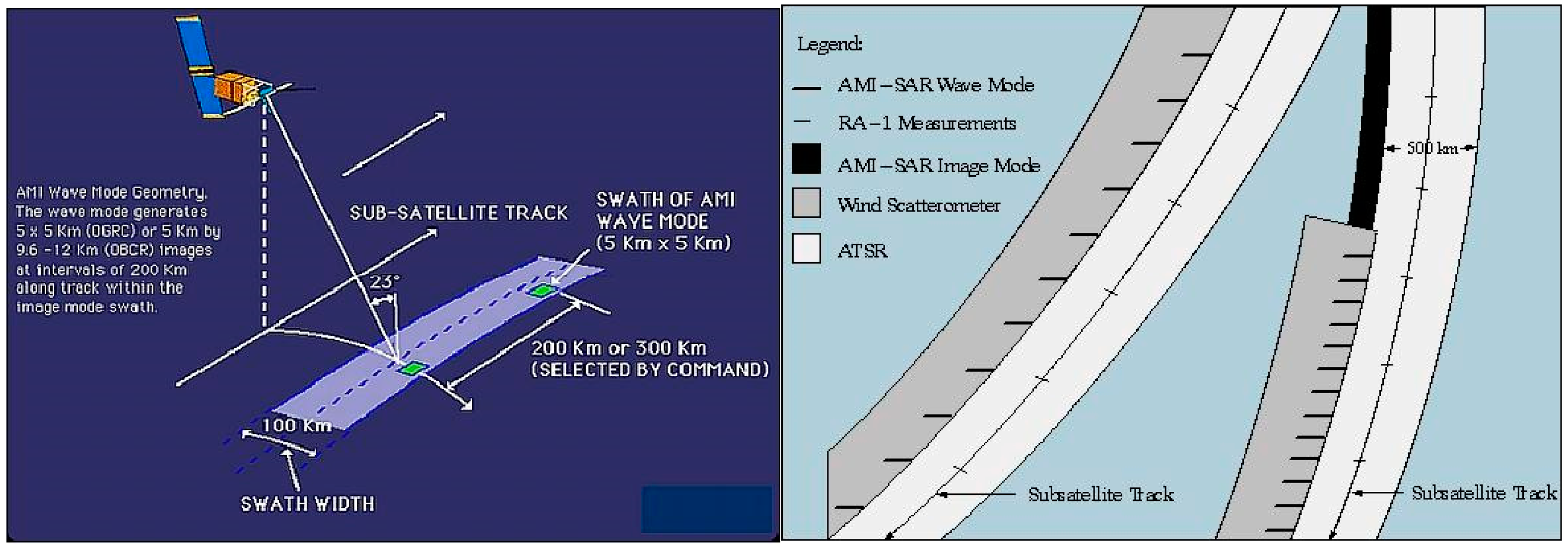
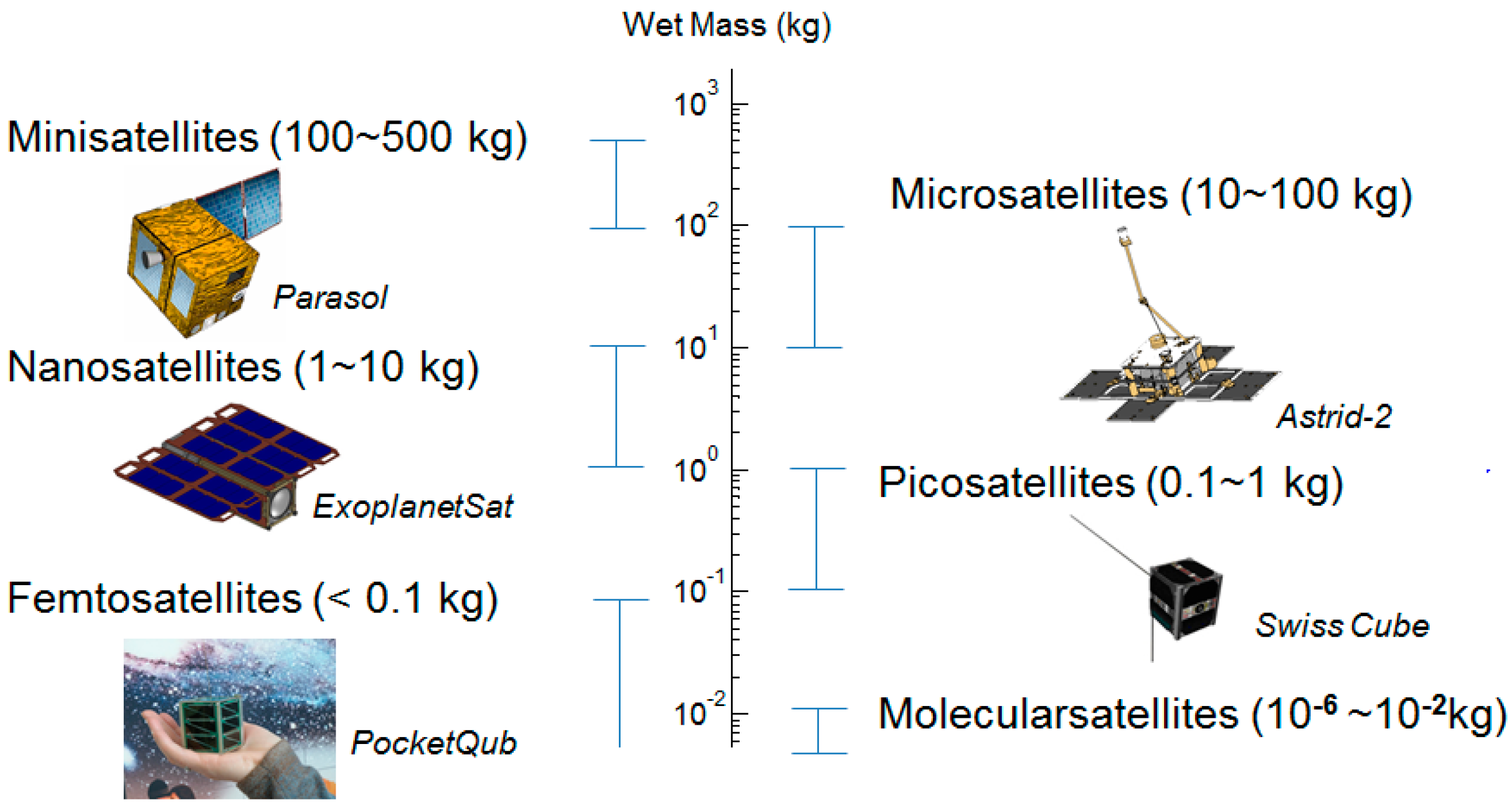
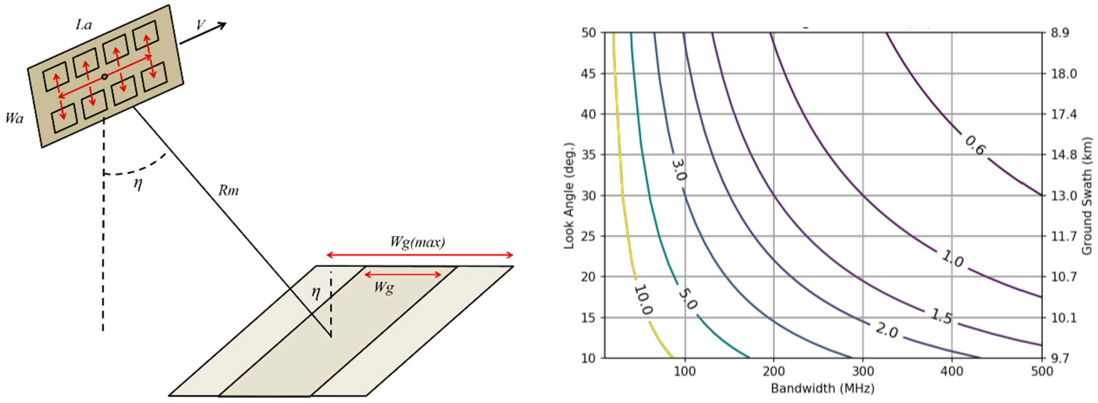
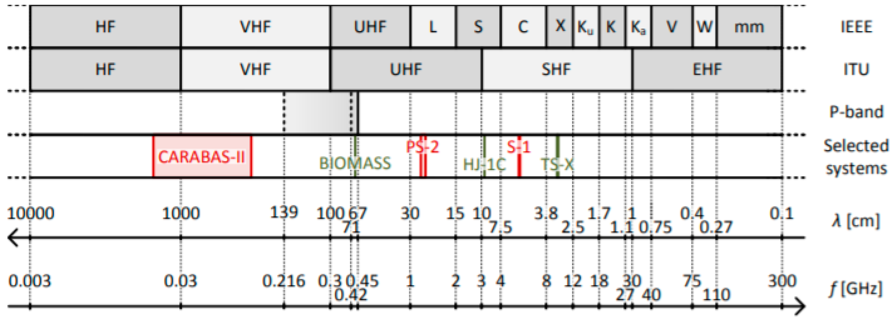
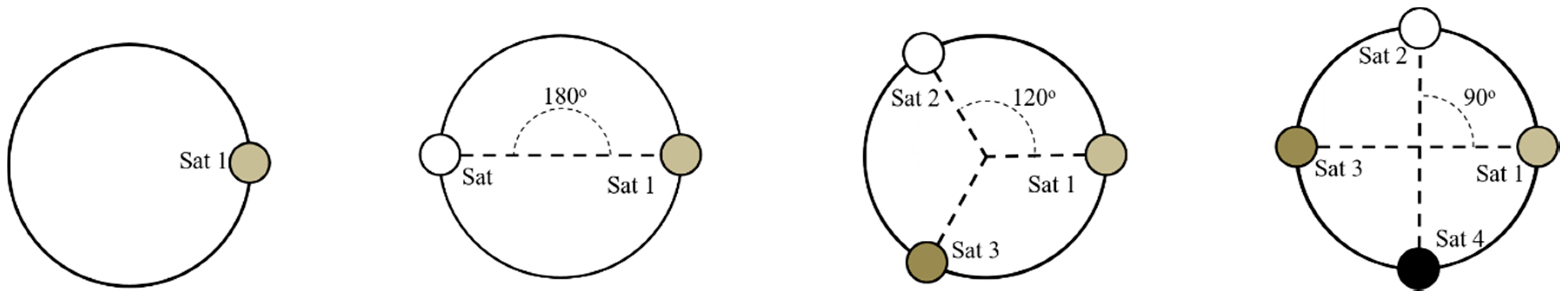
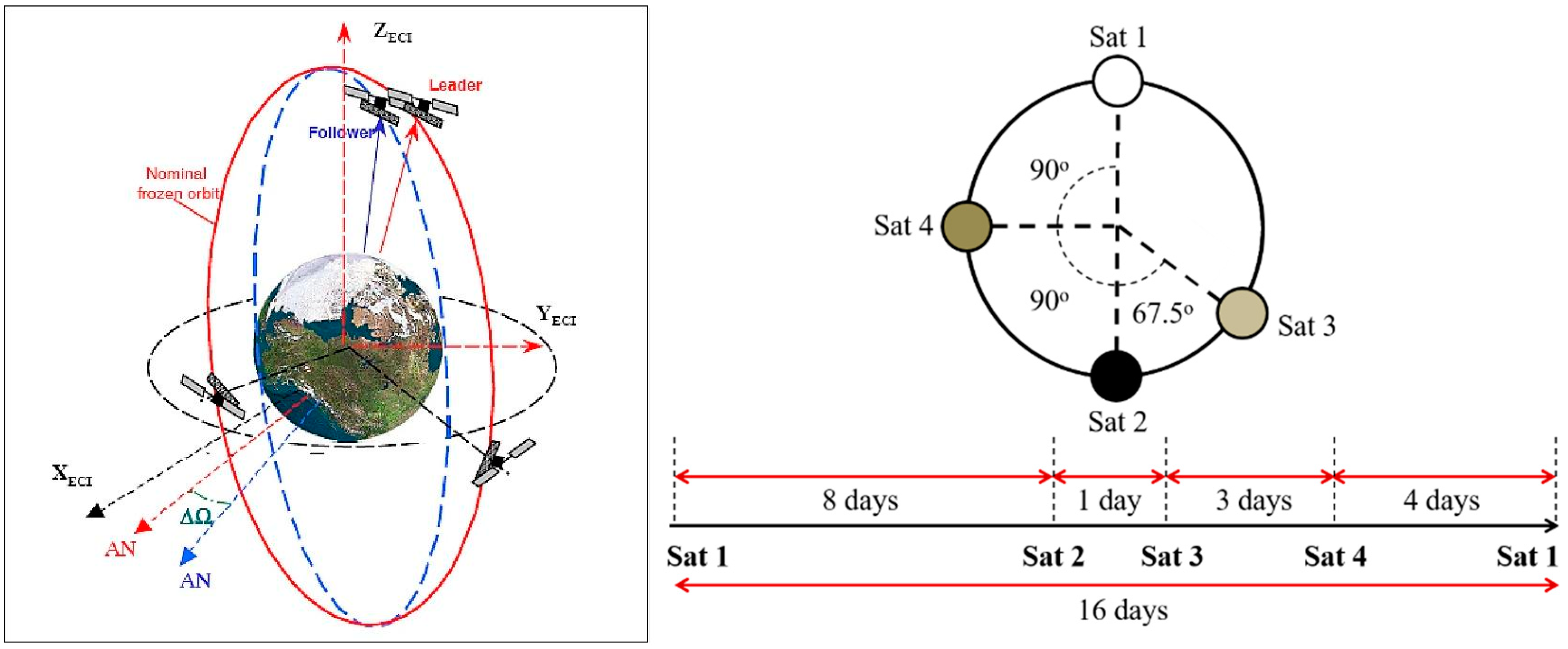
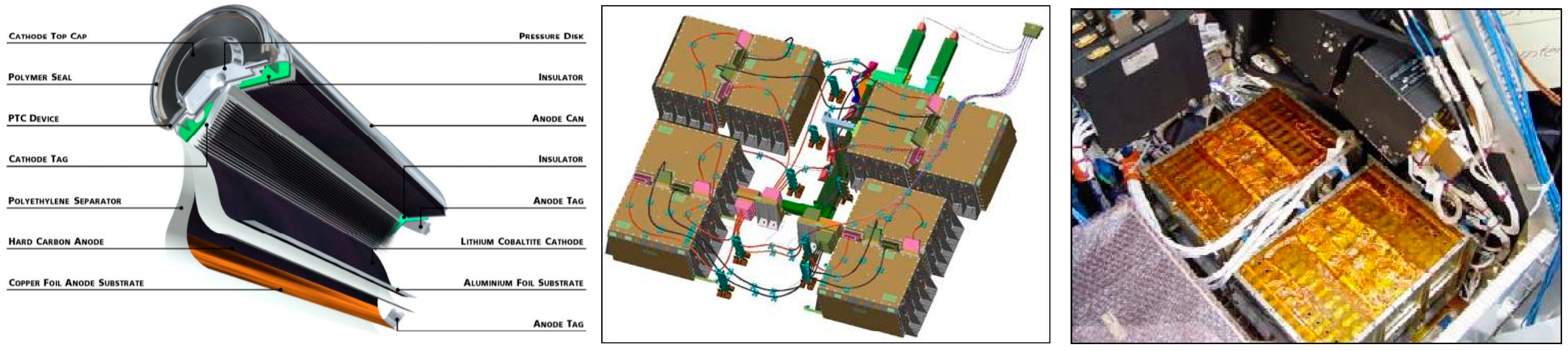
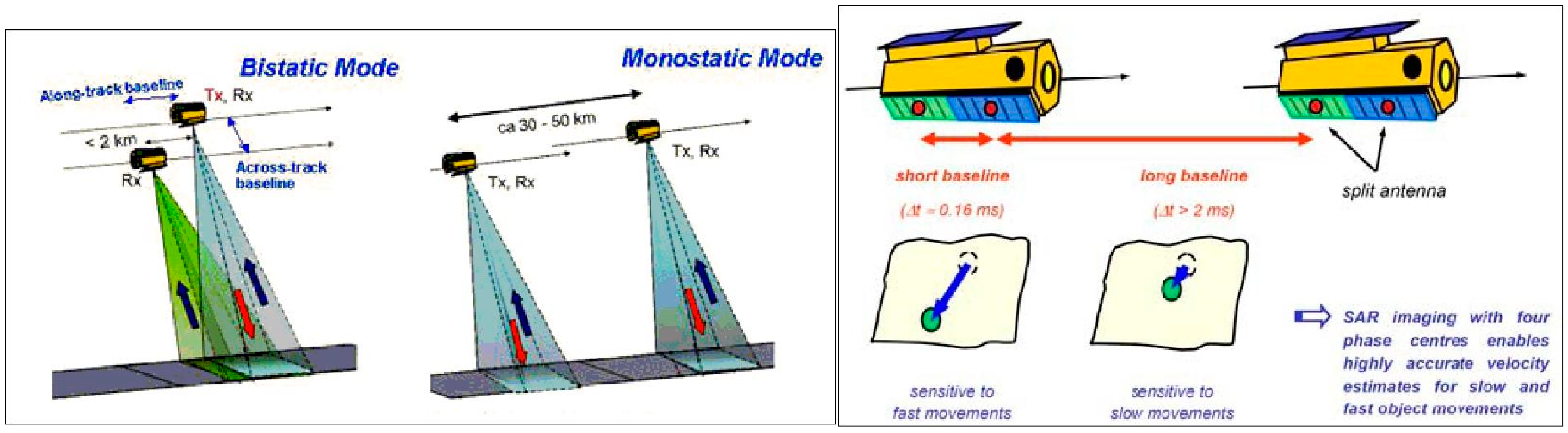
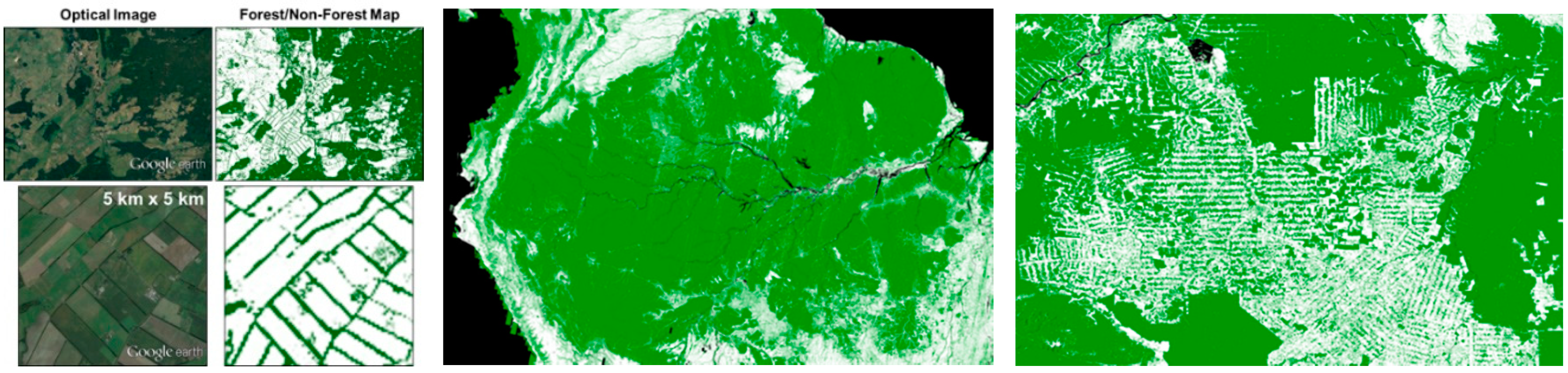
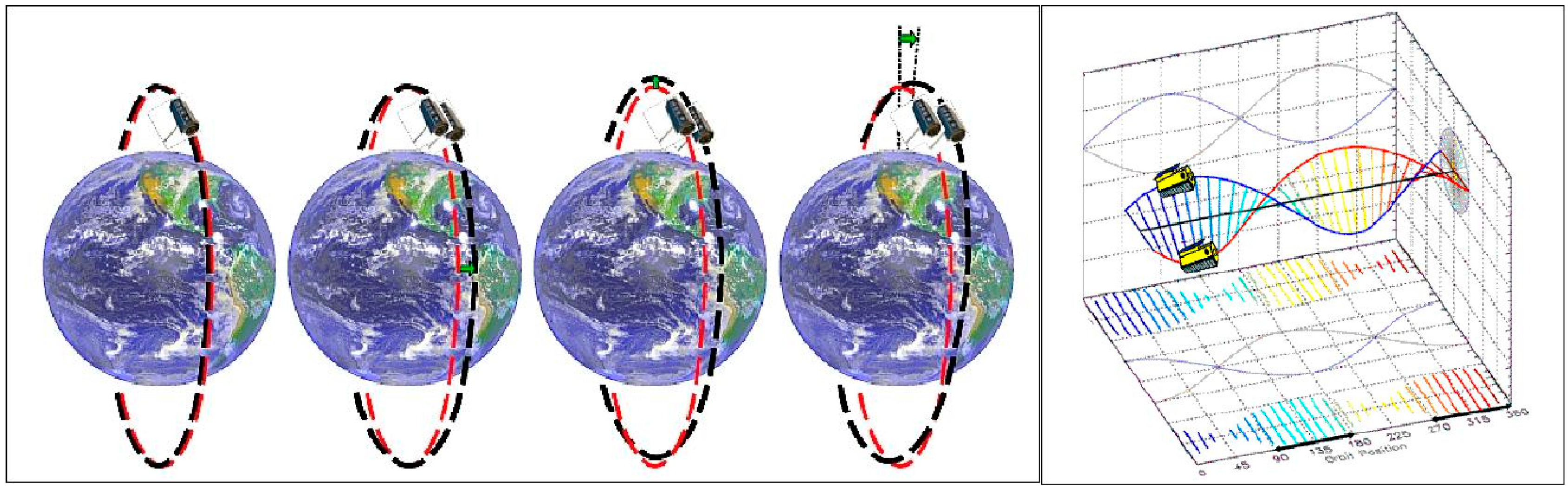
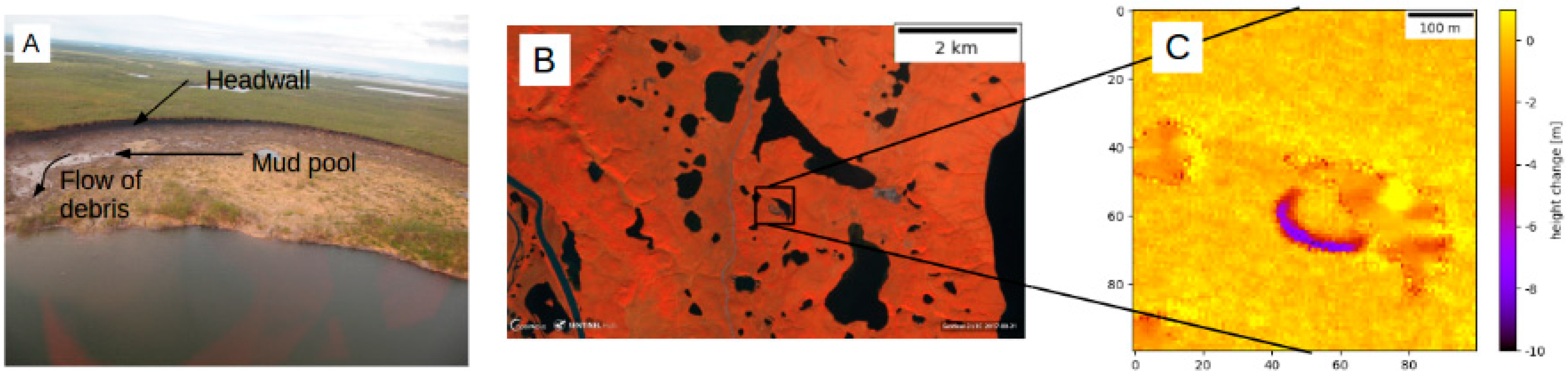
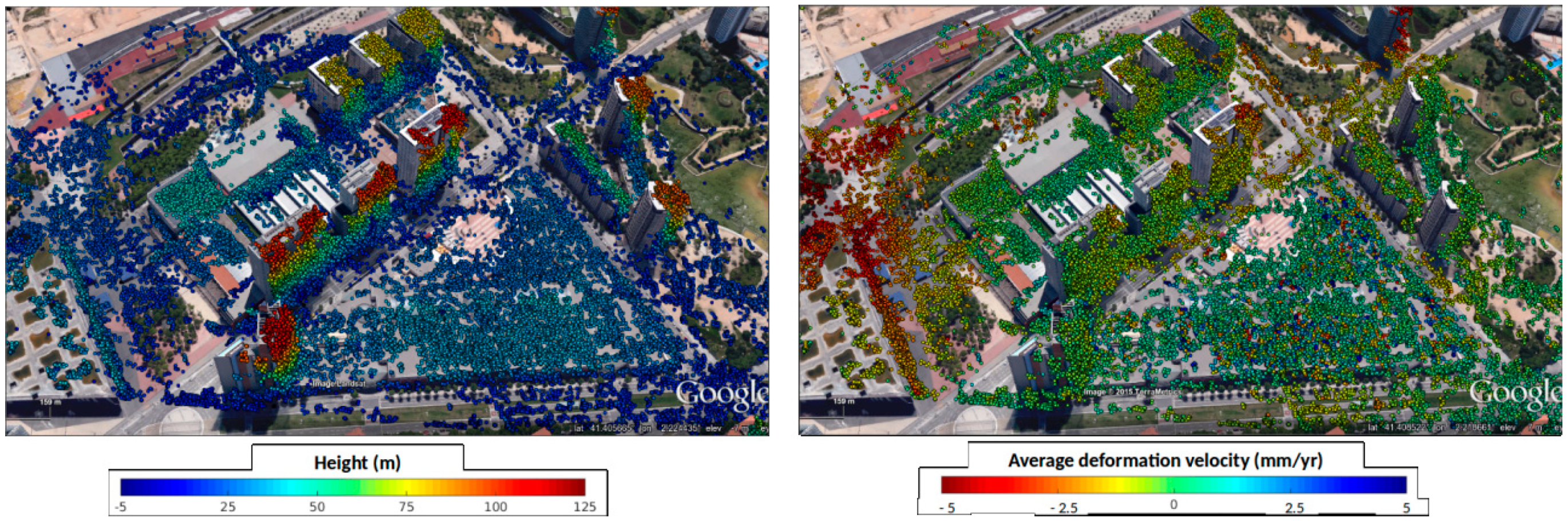
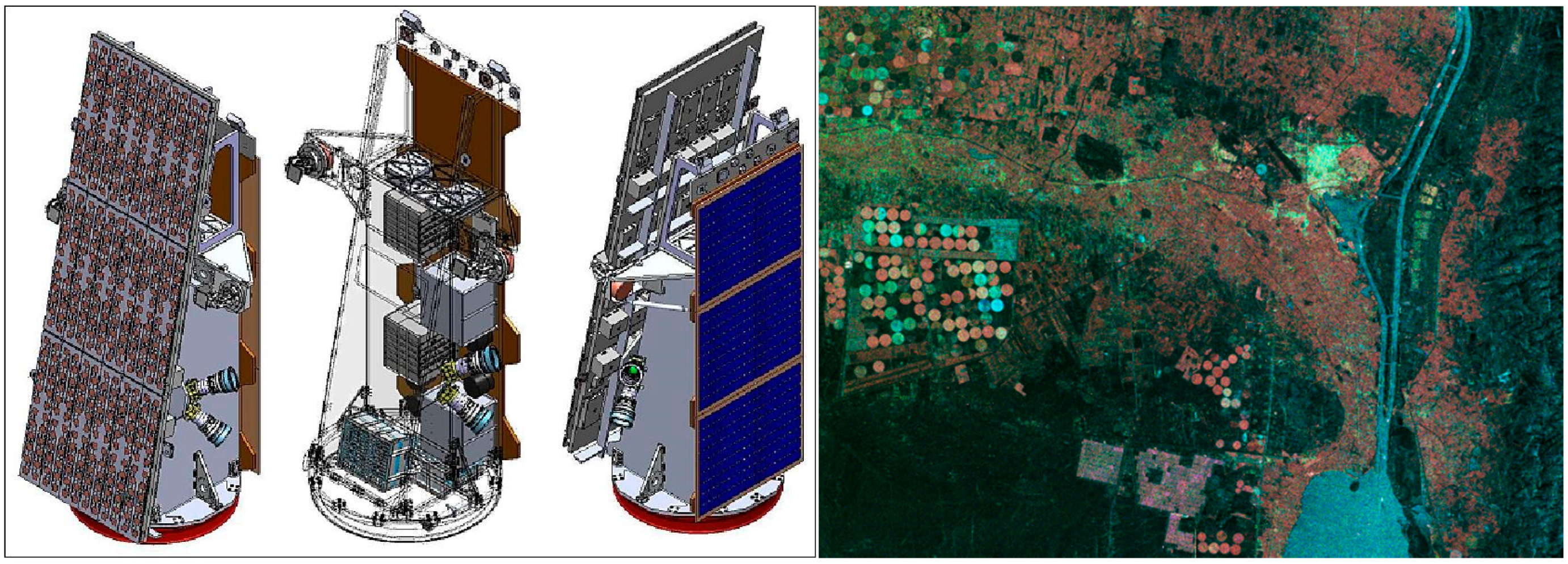
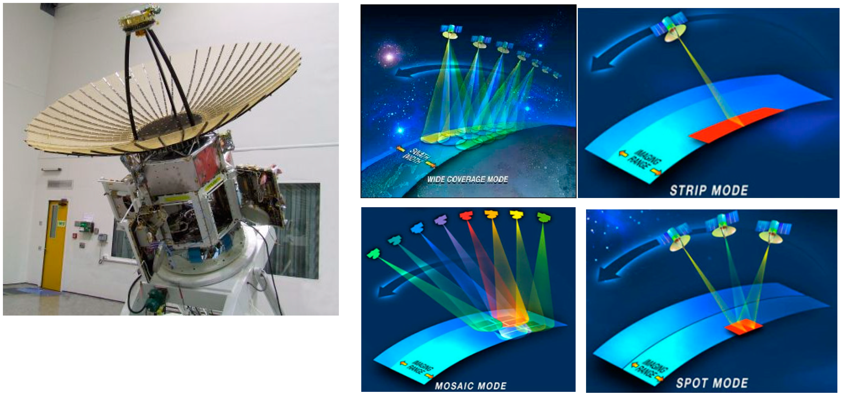
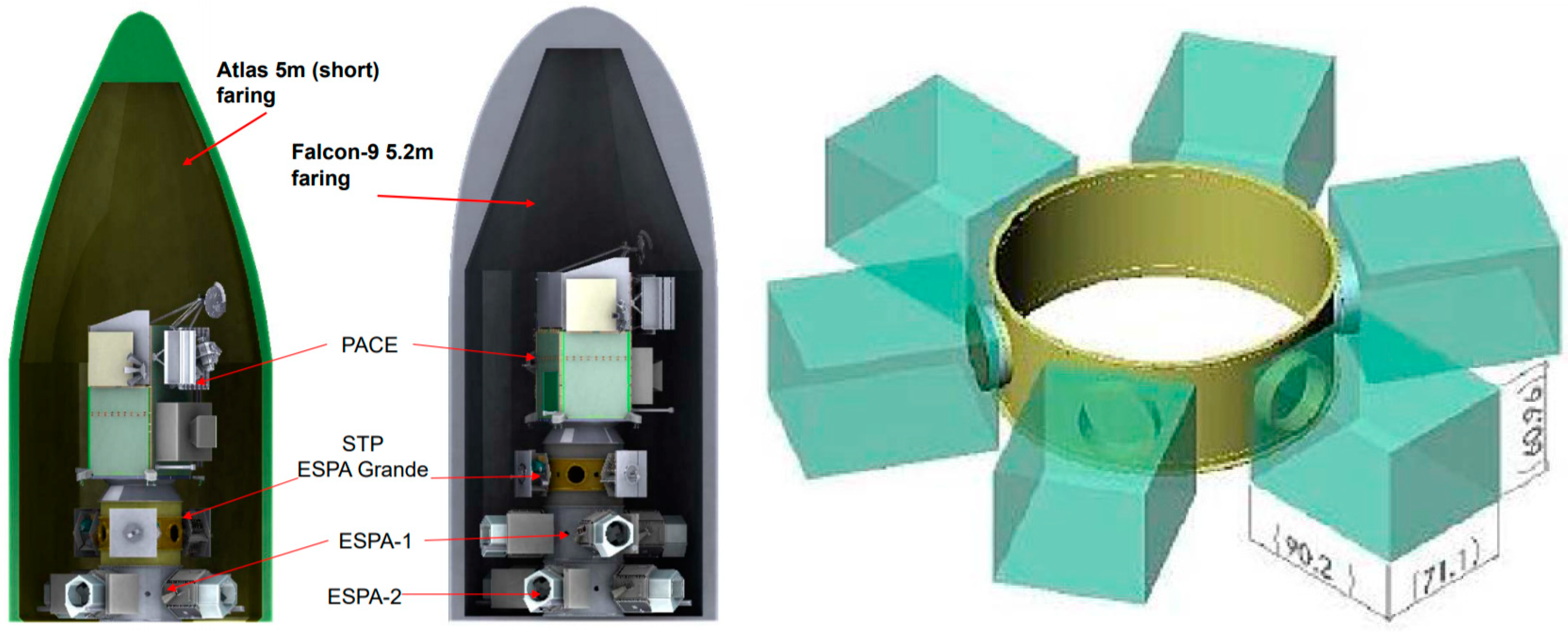
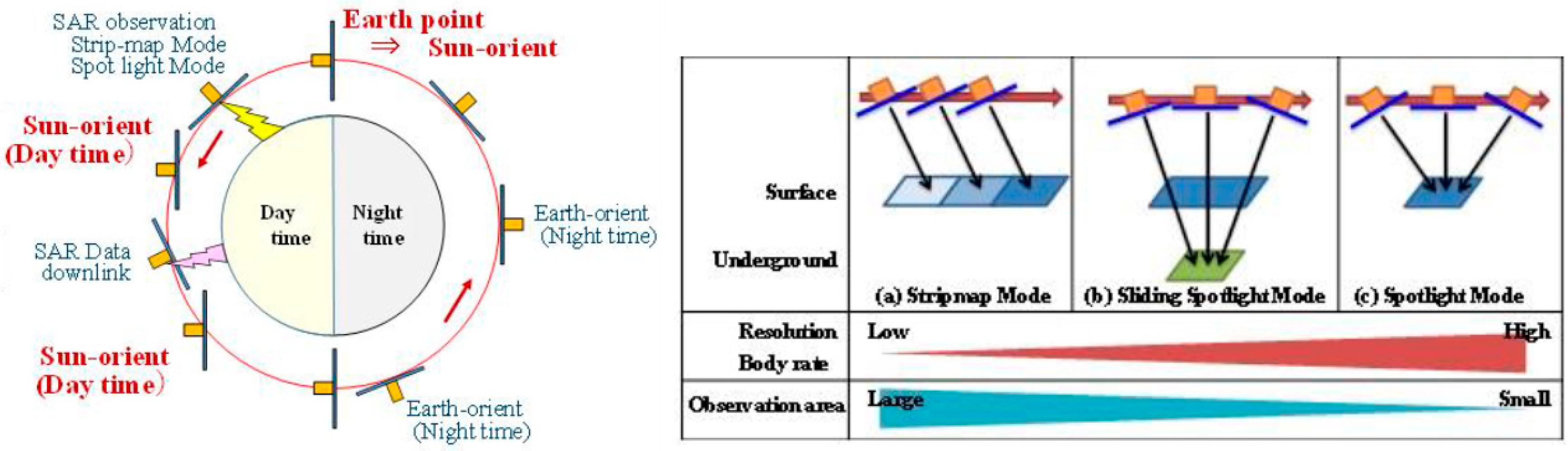
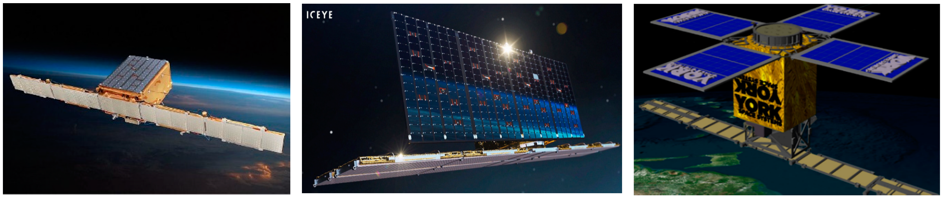
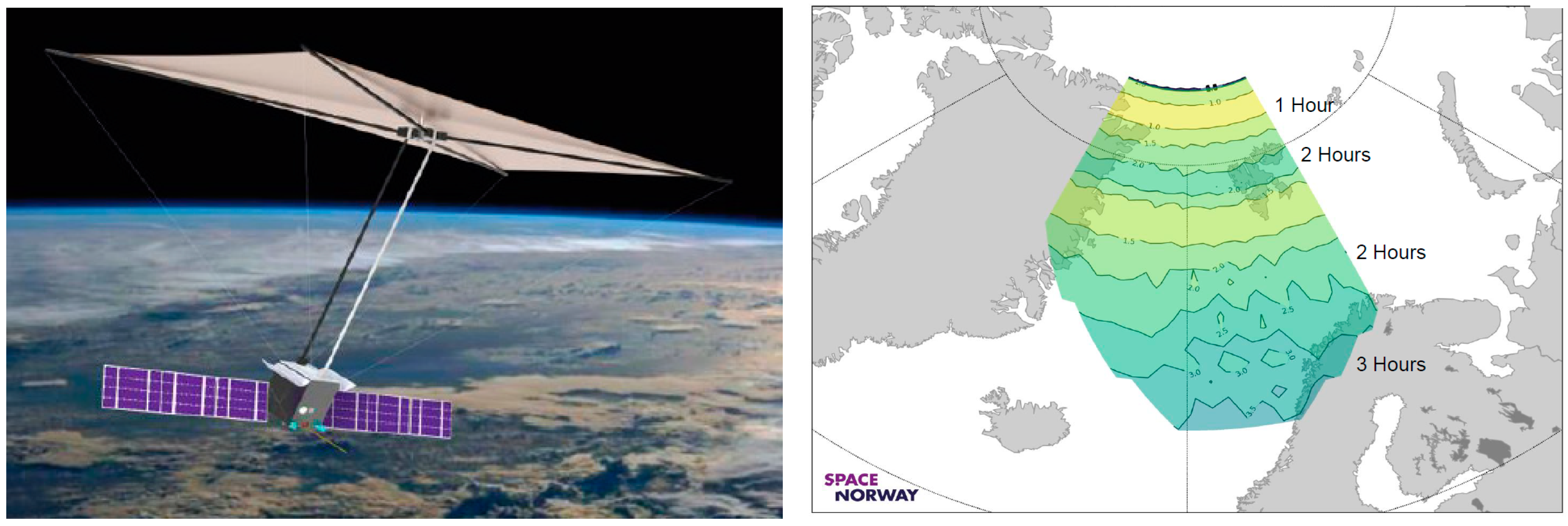
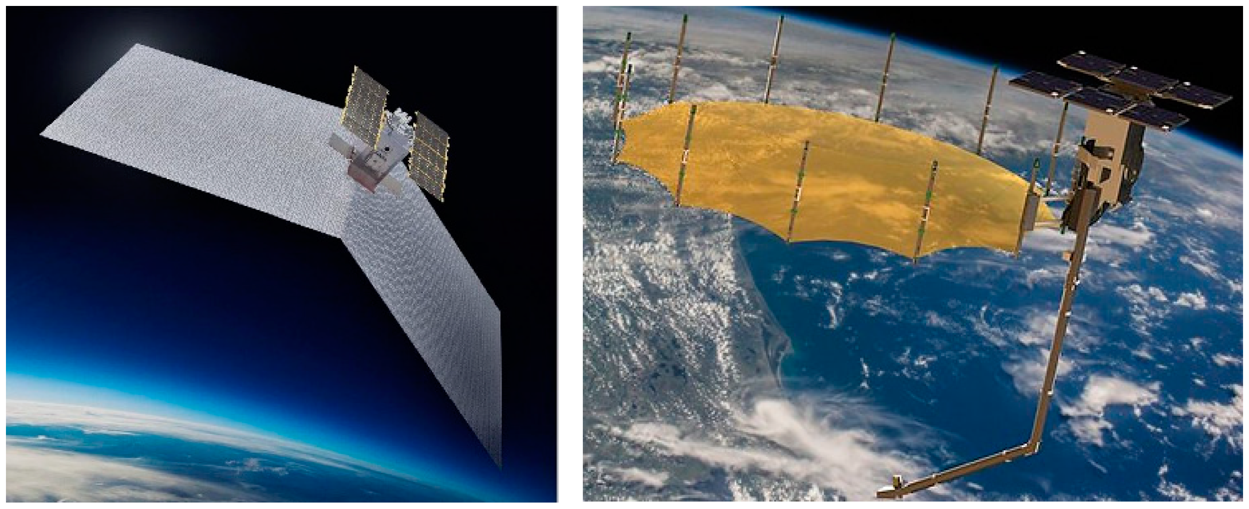
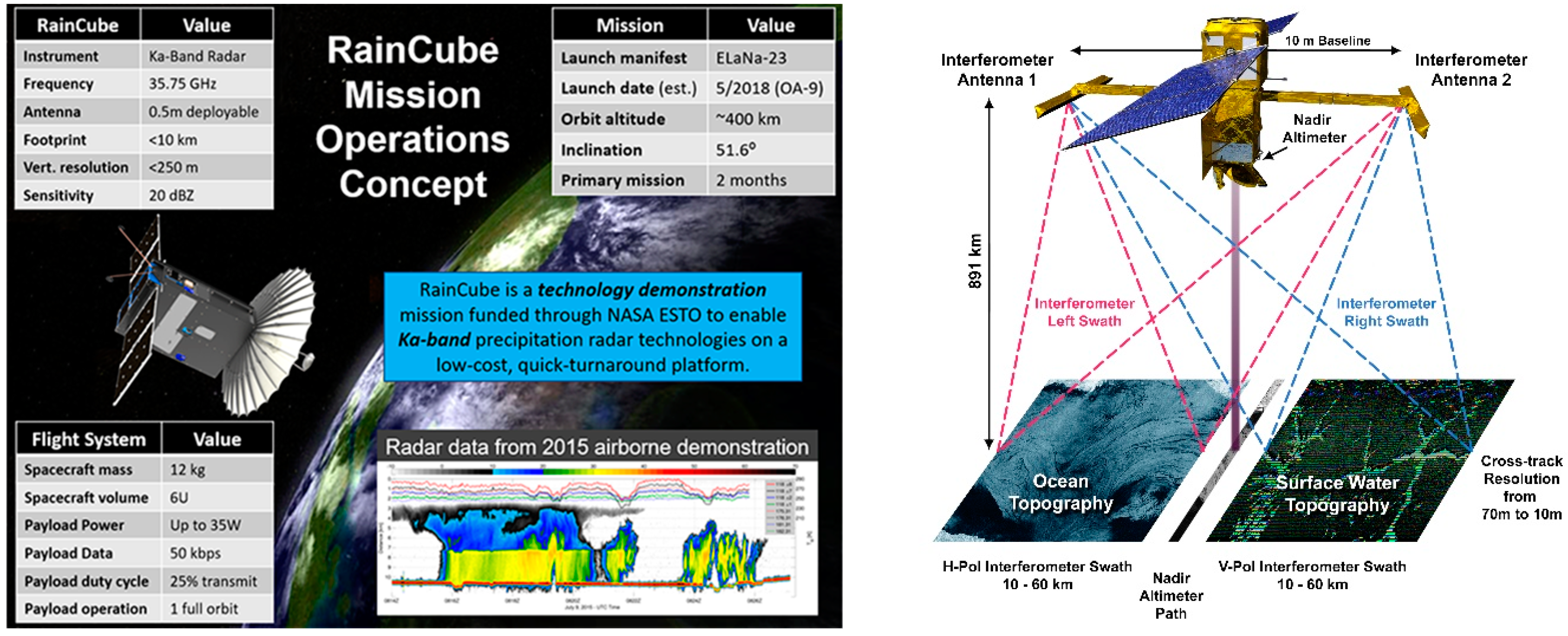
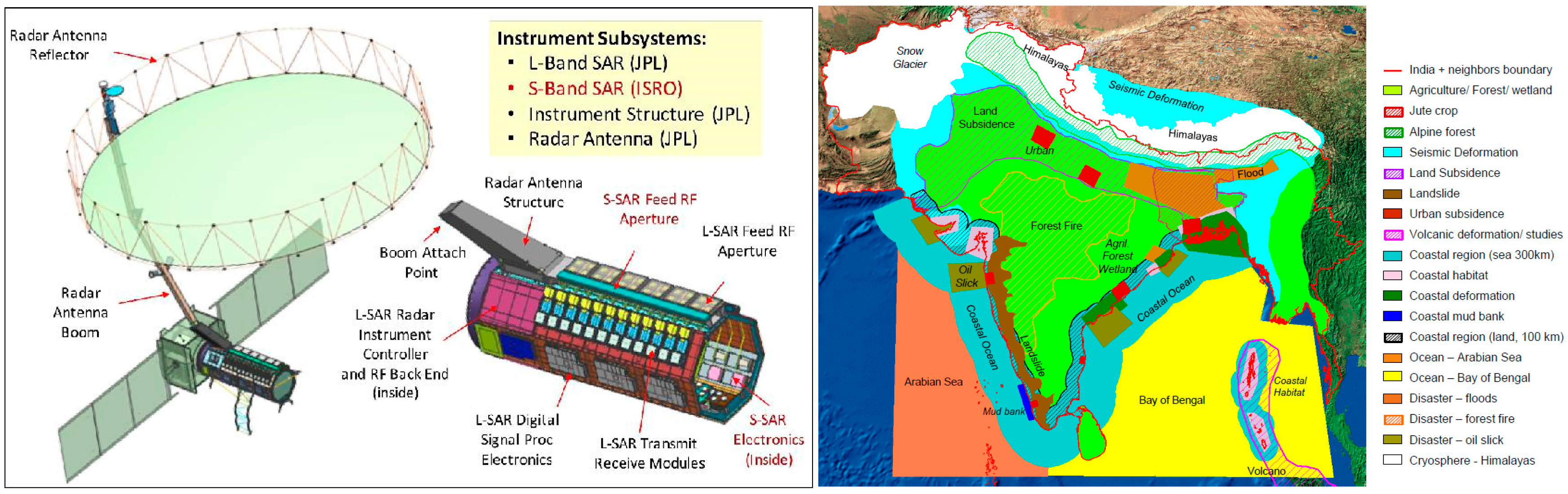
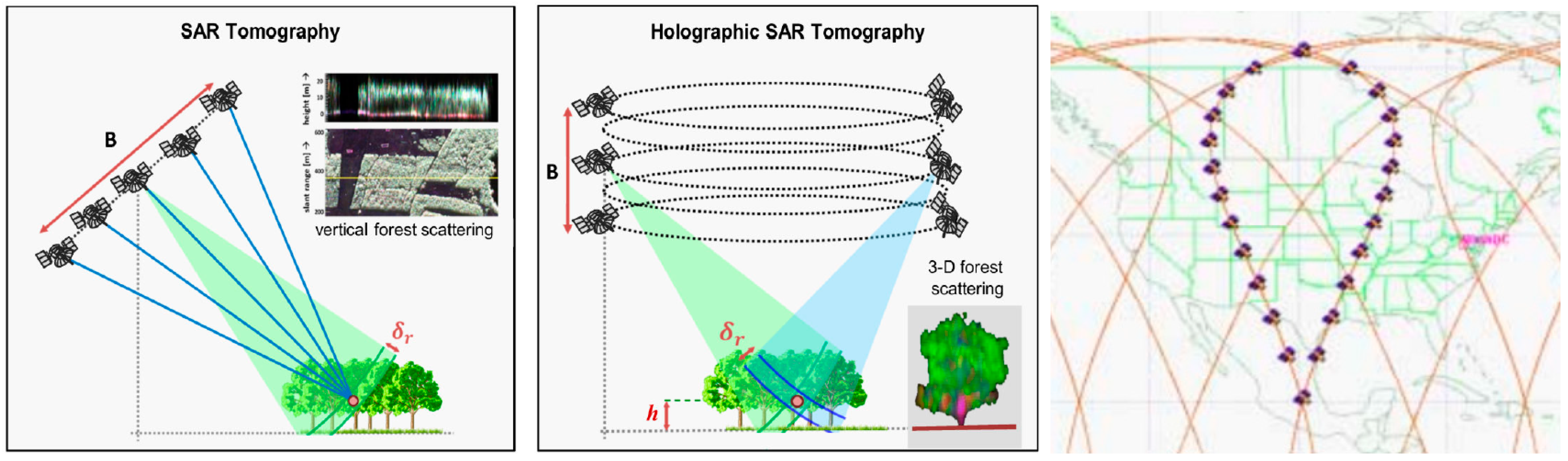
Table 1.
Synthetic aperture radar missions (2018).
| Mission | Country | Duration | Band | Mass (kg) | Swath (km) | Resolution (m, Az-R) |
|---|---|---|---|---|---|---|
| SeaSat | USA | 1978 | L | 2290 | 100 | 6–25 |
| SIR-A1/B1 | USA | 1981, 1984 | L | 2460 | 50 | 7–25/6–13 |
| ERS-1/2 | Europe | 1991–2010 | C | 2384 | 100 | 6–26 |
| 1995–2011 | 2516 | 100 | 6–26 | |||
| ALMAZ-1 | USSR | 1991–1992 | S | 3420 | 280 | 8–15 |
| JERS-1 | Japan | 1992–1998 | L | 1400 | 75 | 18–18 |
| SIR-C/X | Multi 1 | 1994 | C,L/X | 11,000 | 90 | 7.5–13/6–10 |
| RADARSAT-1 | Canada | 1995–2013 | C | 3400 | 500 | 8–8 |
| SRTM1 | Multi 2 | 2000 | C,X | 13,600 | 100 | 15–8/8–19 |
| ENVISAT | Europe | 2002–2012 | C | 8210 | 100 | 6–9 (SM) 3 |
| 405 | 80–8 (SC) 3 | |||||
| ALOS | Japan | 2006–2011 | L | 3850 | 70 | 10–10 (high) |
| 30 | 10–30 (polar) | |||||
| 350 | 100–100 (SC) | |||||
| SAR-Lupe | Germany | 2006– | X | 770 4 | - | - |
| RADARSAT-2 | Canada | 2007–2020 | C | 2200 | 18 | 0.8–1.6 (SL) 5 |
| 100 | 8–9 (std) | |||||
| 500 | 70–70 (SC) | |||||
| Cosmo- | Italy | 2007– | X | 1700 | 10 | 1–1 (SL) |
| SkyMed | 40 | 3–3 (SM) | ||||
| 200 | 30–30 (SC) | |||||
| TerraSAR-X | Germany | 2007–2020 6 | X | 1230 | 10 | 1–1 (SL) |
| 30 | 3–1 (SM) | |||||
| 270 | 40–2 (SC) | |||||
| TecSAR | Israel | 2008– | X | 260 4 | - | - |
| TanDEM-X | Germany | 2009–2020 6 | X | 1230 | - | Same as TSX |
| RISAT-1 | India | 2012–2017 | C | 1860 | 10 | 1–1 |
| 25 | 3–4 | |||||
| 220 | 48–8 | |||||
| HJ-1C | China | 2012–2016 | S | 890 | 100 | 5–20 |
| KOMPSat-5 | S. Korea | 2013–2020 6 | X | 1400 | 18 | 1–1 (high) |
| 30 | 3–3 (std) | |||||
| 100 | 5–5 (wide) | |||||
| Sentinel 1A/B | Europe | 2014– | C | 2300 | 80 | 4–2 (SM) |
| 2016– | 400 | 43–8 (TS) 7 | ||||
| ALOS 2 | Japan | 2014–2020 6 | L | 2120 | 25 | 1–3 (SL) |
| 70 | 5–9 (SM) | |||||
| 490 | 60–45 (SC) | |||||
| PAZ | Spain | 2015– | X | 1230 | 10 | 1–1 (SL) |
| 30 | 3–1 (SM) | |||||
| 100 | 20–20 (SC) | |||||
| RCM | Canada | 2017– | C | 1430 | 20 | 1–1 (SL) |
| 30 | 3–10 (SM) | |||||
| 500 | 40–40 (SC) | |||||
| SAOCOM | Argentina | 2018– | L | 3000 | 30 | 10 (Az, SM) |
| 350 | 100 (Az, TS) |
1 C/L-band: USA, X-band: Germany, Italy; 2 C-band: USA, X-band: Germany; 3 SM: stripmap, SC: ScanSAR; 4 Dry mass; 5 SL: spotlight; 6 World Meteorological Organization (WMO) database; 7 TS: TopSAR.
Table 2.
Areas of research utilizing SAR data. Source: German Aerospace Center (DLR) [25].
Table 2.
Areas of research utilizing SAR data. Source: German Aerospace Center (DLR) [25].
| Category | Application | Temporal Scale | |||
|---|---|---|---|---|---|
| Days | Weeks | Months | Years | ||
| Biosphere | Deforestation or fire | O | O | O | |
| Biodiversity | O | O | O | ||
| Cryosphere | Sea ice | O | O | ||
| Ice cap and glaciers | O | O | |||
| Geosphere | Volcanic activities | O | O | ||
| Seismic activities | O | O | O | O | |
| Landslides | O | O | |||
| Hydrosphere | Floods and soil moisture | O | O | ||
| Ocean currents and tides | O | O | |||
Table 3.
Revisit time of Cosmo-SkyMed during constellation deployment.
| Configuration | Average Revisit Time, h | Worst Revisit Time, h | ||
|---|---|---|---|---|
| # Satellites | Left and Right | Right | Left and Right | Right |
| 1 | 18 to 35 1 (12 to 23) 2 | 37 to 64 (25 to 44) | 156 (60) | 252 (120) |
| 2 | 9 to 18 (6 to 12) | 19 to 35 (13 to 24) | 60 (36) | 108 (60) |
| 3 | 6 to 12 (4 to 8) | 13 to 24 (9 to 16) | 36 (36) | 60 (36) |
| 4 | 5 to 9 (3 to 6) | 10 to 18 (6 to 12) | 24 (12) | 60 (24) |
1 Nominal; 2 Extended.
Table 4.
Areal coverage response of Cosmo-SkyMed during constellation deployment.
| Configuration | Coverage After 12 h, % | Coverage After 24 h, % | ||
|---|---|---|---|---|
| # Satellites | Left and Right | Right | Left and Right | Right |
| 1 | - | - | 67 (85) | 38 (55) |
| 2 | 62 1 (84) 2 | 41 (62) | 81 (92) | 64 (84) |
| 3 | 88 (98) | 62 (84) | 96 (99.97) | 84 (98) |
| 4 | 97 (100) | 80 (99) | 100 (100) | 95 (100) |
1 Nominal; 2 Extended.
Table 5.
NovaSAR observation modes and 1-satellite/3-satellite revisit performance.
| Observation Mode | Resolution (m) | Swath (km) | Look Angle (°) | Av. Revisit Time (Day) | Max. Revisit Time (Day) |
|---|---|---|---|---|---|
| 1. ScanSAR | 20 m | 50–100 | 16–30 | 3.7 (1.5), 2.5× | 14 (3.5), 4× |
| 2. Maritime surveillance | 30 m | 750 | 48–73 | 0.9 (0.3), 3.0× | 8 (0.5), 16× |
| 3. Stripmap | 6 m | 13–20 | 16–31 | 3.2 (1.1), 2.9× | 12.5 (3.5), 3.4× |
| 4. ScanSAR wide | 30 m | 55–140 | 15–32 | 3.7 (1.2), 3.1× | 13 (3.5), 3.7× |
Table 6.
Power and mass of different SAR missions from nanosatellites to medium satellites.
| Mission | Battery Capacity | Solar Array Power | Payload Peak Power | Payload Mass | Total Launch Mass |
|---|---|---|---|---|---|
| RaInCube | ~10 Ah | 45 W | 22 W | 5.5 kg | 12 kg |
| TECSAR | 45 Ah | 1600 W | 850 W | 100 kg | 260 kg |
| HJ-1C | 80 Ah | 1100 W | - | 200 kg | 890 kg |
| SAR-Lupe | 108 Ah | - | 1800 W | 394 kg | 1230 kg |
| TSX | 132 Ah | - | - | - | 770 kg |
| Cosmo-SkyMed | 336 Ah | 40,000 W | 7000 W | - | 1700 kg |
Table 7.
Capella X-SAR observation modes and 1-satellite/3-satellite revisit performance.
| Total # Satellites → | 6 | 12 | 24 | 36 |
|---|---|---|---|---|
| # orbit planes | 2 | 4 | 8 | 12 |
| Average revisit (h) | <4 | <2 | 1 | <1 |
| Maximum revisit (h) | 12 | 6 | 4 | <2 |
| InSAR revisit (h) | 24 | 12 | 6 | 4 |
Table 8.
Comparison of NISAR, Tandem-L, and NovaSAR missions (~2018).
| Mission | NISAR | Tandem-L | NovaSAR | |||
|---|---|---|---|---|---|---|
| # Sats (→) Orbit (inc) | 1 SSO (98.4°) | 2 SSO (98.4°) | 1 SSO (97.5°) | EqO (15°) | 3 SSO (97.5°) | EqO (15°) |
| Altitude | 747 km | 745 km | 580 km | (←) | (←) | (←) |
| LTAN | 18:00 h | - | 10:30 h | (←) | (←) | (←) |
| Repeat cycle | 12 day | 16 days | - | - | - | - |
| Revisit time | 5–7 day | 3–4 day | 1–3 day | 0.5–1.5 day | 0.5–1.5 day | 0.3 day |
| Band | S, L | L | S | (←) | (←) | (←) |
| Resolution | 7 m (Az), | 7 m, | 6–30 m | (←) | (←) | (←) |
| 3–24 m (SR) | 1 m (Spot) | (←) | (←) | (←) | ||
| Swath | 240 + km | 350 km | 20–150 km | (←) | (←) | (←) |
Table 9.
Tandem-L requirements in biosphere monitoring.
| Application | Resolution (Global/Local) | Accuracy |
|---|---|---|
| Upper canopy height and change | 50 m/30 m | 10% error for height <2 m |
| 3D forest structure and change | 50 m/30 m | - |
| Forest biomass and change | 100 m/50 m | 20% error for biomass <100 ton/ha |
| Agricultural SAR products | 40 m | - |
Table 10.
NovaSAR observation modes and 1-satellite/3-satellite revisit performance [41].
Table 10.
NovaSAR observation modes and 1-satellite/3-satellite revisit performance [41].
| Mission | Cost/kg (kUSD) | Sat Mass (kg) | Sat Cost (MUSD) | Launch Cost (%) | Launch Vehicle | Ground Station |
|---|---|---|---|---|---|---|
| ICEYE | 82 | 85 | 7 | 42 | Falcon 9, Electron | KSAT |
| SAR-Lupe | 117 | 770 | 90 | 24 | Kosmos | DLR |
| TSX/TDX | 143 | 1230 | 117 | 20 | Dnepr | DLR |
| NovaSAR | 146 | 400 | 59 | 23 | PSLV | KSAT |
| Capella | 163 | 48 | 8 | 21 | Falcon 9, PSLV, Electron | AWS |
| X-SAR | ||||||
| Cosmo-SkyMed | 214 | 1700 | 364 | 13 | Soyuz | KSAT |
© 2020 by the authors. Licensee MDPI, Basel, Switzerland. This article is an open access article distributed under the terms and conditions of the Creative Commons Attribution (CC BY) license (http://creativecommons.org/licenses/by/4.0/).
Share and Cite
MDPI and ACS Style
Paek, S.W.; Balasubramanian, S.; Kim, S.; de Weck, O. Small-Satellite Synthetic Aperture Radar for Continuous Global Biospheric Monitoring: A Review. Remote Sens. 2020, 12, 2546. https://doi.org/10.3390/rs12162546
AMA Style
Paek SW, Balasubramanian S, Kim S, de Weck O. Small-Satellite Synthetic Aperture Radar for Continuous Global Biospheric Monitoring: A Review. Remote Sensing. 2020; 12(16):2546. https://doi.org/10.3390/rs12162546
Chicago/Turabian StylePaek, Sung Wook, Sivagaminathan Balasubramanian, Sangtae Kim, and Olivier de Weck. 2020. "Small-Satellite Synthetic Aperture Radar for Continuous Global Biospheric Monitoring: A Review" Remote Sensing 12, no. 16: 2546. https://doi.org/10.3390/rs12162546
Note that from the first issue of 2016, this journal uses article numbers instead of page numbers. See further details here.