
CFD Turbulence Models Assessment for the Cavitation Phenomenon in a Rectangular Profile Venturi Tube
by
 , and
, and
Mauricio De la Cruz-Ávila
1,2,*,
Jorge E. De León-Ruiz
3,
Ignacio Carvajal-Mariscal
4 and
and
Jaime Klapp
1,* 1
Instituto Nacional de Investigaciones Nucleares, ININ, Carretera México Toluca-La Marquesa s/n, Ocoyoacac 52750, Mexico
2
Centro de Investigación y de Estudios Avanzados, CINVESTAV, Instituto Politécnico Nacional 2508, San Pedro Zacatenco, Mexico City 07360, Mexico
3
Centro de Investigación en Materiales Avanzados, S.C., CIMAV, Complejo Industrial Chihuahua, Miguel de Cervantes 120, Chihuahua 31136, Mexico
4
Instituto Politécnico Nacional, ESIME—UPALM, Mexico City 07738, Mexico
*
Authors to whom correspondence should be addressed.
Fluids 2024, 9(3), 71; https://doi.org/10.3390/fluids9030071
Submission received: 5 October 2023
/
Revised: 16 December 2023
/
Accepted: 17 December 2023
/
Published: 7 March 2024
(This article belongs to the Special Issue Pipe Flow: Research and Applications)
Abstract
:This study investigates cavitation in a rectangular-profile Venturi tube using numerical simulations and four turbulence models. The unsteady Reynolds-averaged Navier–Stokes technique is employed to simulate vapor cloud formation and compared against experimental data. κ-ε realizable, κ-ε RNG, κ-ω SST, and κ-ω GEKO models are evaluated. The simulation results are analyzed for pressure, turbulence, and vapor cloud formation. Discrepancies in cavitation cloud formation among turbulence models are attributed to turbulence and vapor cloud interactions. RNG and SST models exhibit closer alignment with the experimental data, with RNG showing a superior performance. Key findings include significant vapor cloud shape differences across turbulence models. The RNG model best predicts velocity at the throat exit with an error of 4.145%. Static pressure predictions include an error of 4.47%. The vapor cloud length predictions show variation among models, with the RNG model having a 0.386% error for the minimum length and 4.9845% for the maximum length. The SST model exhibits 4.907% and 13.33% errors for minimum and maximum lengths, respectively. Analysis of the cavitation number reveals agreement with the experimental data and sensitivity to cavitation onset. Different turbulence models yield diverse cloud shapes and detachment points. Weber number contours illustrate the variation in the cavitation cloud behavior under different turbulence models.
Keywords:
turbulence model κ-ε RNG; κ-ε realizable; κ-ω SST; κ-ω GEKO; cavitation; Venturi tube; vapor cloud1. Introduction
The formation of vapor bubbles in a liquid due to a pressure drop is known as the cavitation phenomenon. This is a hydrodynamic phenomenon that occurs when the fluid pressure decreases enough to create vapor bubbles. These bubbles can rapidly collapse and create shock waves that damage the surrounding surfaces. It is a common problem in industrial and engineering applications, and can cause a loss of efficiency, increased noise, and equipment damage.
Many hydrodynamic applications, hydraulic systems, and turbo-machinery exhibit this behavior. They are classified as external or internal flow, as well as total or partial cavitation. For internal flow, such as hydro turbines [1], diesel injectors [2,3], or sudden contraction pipes [4], partial cavitation [5,6] is connected with a periodic shedding of significant vapor clouds [7], which causes erosion [8]. The most commonly observed form is partial cavitation, which occurs when the cavity closes on the surfaces of a flow obstruction. It eventually causes structural damage and affects the surface performance of the equipment. Such implications have motivated the analysis of different forms of cavitation, and great efforts have been made to understand the dynamics of partial cavitation in particular. These cavitation pockets are characterized by an oscillating closure zone [9], which causes cavity length oscillations [10,11] and vapor structure shedding [12]. Depending on the flow in the cavity closure zone, the partial cavity [13] can take one of two forms: a closed or quasi-stable cavity and an open cavity or cloud cavitation. With a relatively steady cavity length, a quasi-stable cavity exhibits only minor shedding near its closure zone. A cavitation cloud, on the other hand, is a very unstable event with a periodically fluctuating length linked with massive vapor cloud shedding [14]. This variety of cavities has been examined experimentally [15,16,17,18] and computationally [7,19,20] in order to understand the physical process, internal cavity structure, and turbulence–cavitation interaction, as well as to study the transition from quasi-stable to a cavitation cloud.
Numerical simulations based on the Navier–Stokes framework are widely used to predict cavitation. These simulations model the fluid dynamics and incorporate turbulence models to predict the formation and collapse of cavitation bubbles. Turbulence models, based on the Reynolds-averaged Navier–Stokes (RANS) technique, are particularly common for predicting cavitation. The accuracy and efficiency of these simulations depend significantly on the selection of a suitable turbulence model. The RANS models are widely accepted and computationally efficient for simulating industrial flows. They solve for time-averaged flow variables and rely on a turbulence closure model to account for turbulence fluctuations. The proper selection of turbulence models is crucial for accurate prediction of flow field, pressure distribution, and cavitation behavior.
Various RANS turbulence models have been employed to simulate the cavitation phenomenon, each with its own advantages and limitations. The most prominent models include the standard [21,22], the realizable [23,24], the renormalization group (RNG) [25], the shear stress transport (SST) [26,27], and the generalized (GEKO) [28]. The standard model is the simplest and most widely used turbulence model, but it has limitations in capturing complex flow features, such as separation, recirculation, and swirling flow. The realizable improves upon the standard model by accounting for the effects of streamline curvature and pressure-strain, but it is still limited in complex flow cases. The RNG further improves upon the realizable by incorporating an extra term for anisotropy and enhancing the turbulence transport. The model is another commonly used turbulence model, which has a better prediction capability in near-wall regions and complex flows. The SST combines the benefits of the and models and has been widely used in simulating turbulent flows with separation and recirculation. The GEKO is a relatively new turbulence model, which has shown promising results in simulating high-speed flows and cavitation. The RNG model is useful for predicting cavitation, which uses renormalization theory to account for turbulence effects at different scales. This model has the ability to predict both the formation and collapse of cavitation bubbles and can also predict the transition from a turbulent boundary layer to a laminar boundary layer, which is important for predicting bubble formation in the cavitation region. However, it has been observed that the RNG model may have lower accuracy in predicting flows with separation and recirculation.
On the other hand, the RLZ model uses a transport equation for turbulent stress that takes into account physical constraints and can accurately predict the boundary layer separation. However, the model may underestimate turbulence production and does not account for the presence of cavitation bubbles in the simulation.
The SST model uses two different equations for the turbulent kinematic viscosity in the boundary layer and in the core of the flow, allowing for accurate prediction of the transition from a laminar to a turbulent boundary layer. Additionally, the SST model is capable of predicting boundary layer separation and can be used in a wide range of applications. However, the model may be less accurate in predicting highly turbulent flows and may underestimate turbulence production.
Finally, the GEKO model uses a transport equation for kinematic turbulence and a transport equation for turbulent stress, allowing a better representation of boundary layer turbulence. Additionally, this model has an adjustment parameter that allows a more precise adaptation of the wall slope, making it more suitable for solving problems that require a high degree of detail in the boundary layer. However, a significant disadvantage is its complexity. Due to the inclusion of an additional transport equation for turbulent stress, the GEKO model requires more computational resources than the other turbulence models. Additionally, the choice of the adjustment parameter can be complicated and may require careful calibration to obtain accurate results. Therefore, the GEKO model may not be the best choice in situations where fast simulation is required or where limited computational resources are available.
Coutier-Delgosha et al. [29] carried out a study on the unsteady effects associated with cavitation by conducting 2D numerical simulations in three different cavitating systems. Various turbulence models were compared, and it was found that both the RNG and turbulence models, with corrections for compressibility effects, were consistent with the available experimental data. The ability of the proposed physical cavitation model, associated with either of these two turbulence models, to predict the unsteady behavior of cavitation sheets was confirmed through two complementary test cases. However, their findings were limited by the fact that the simulations were in 2D, due to the high computational demand of calculation.
The performance of the SST and turbulence models in simulating cavitation in a Venturi tube was evaluated by Chebli et al. [30]. The authors found that the SST model produced more accurate results than the model, particularly in predicting the location of cavitation inception. They noted that the SST model was better suited for simulating the cavitation phenomenon in a Venturi tube due to its ability to model the effects of turbulence on the formation of the sheet cavity. Subsequently, Chebli et al. [31] compared the performance of different turbulence models, such as the RNG and SST models, for predicting cavitating flows in hydrofoils. The results showed that both the SST and RNG models provided good agreement with the experimental data. Additionally, an adapted modification of the turbulent viscosity produced even better cavity results. The study concluded that the SST model is the most suitable turbulence model for simulating cavitating flows in hydrofoils.
In a recent study [32], the performance of the SST, , and Spalart–Allmaras [33] turbulence models was compared in simulating cavitation in a Venturi tube. The authors found that a four-equation adaption for any model produced the most accurate results when compared to experimental data. They noted that the Spalart–Allmaras model was not suitable for simulating cavitation in a Venturi tube due to its inability to accurately model turbulence. In fact, the results are not quite precise to represent a 3D model due to this formulation being developed for 2D simulation models.
Fadaei-Roodi and Pasandidehfard [34] conducted a numerical study on the cavitating flow around cylindrical projectiles with flat or hemispherical heads. Four turbulence models were used in combination with the Zwart cavitation model: realizable, standard, SST, and GEKO. The aim was to predict the cavity dimensions, pressure distribution, and flow dynamics inside and around the cavity, specifically at the closing point. They concluded that the GEKO turbulence model outperforms other turbulence models, SST, standard, and realizable, for predicting the cavitating flows around cylinders of flat and round heads. The study shows that the GEKO model predicts the results much better, especially for higher cavitation number values, and is considered the most suitable turbulence model for numerical simulation.
He and Bai’s research [35] focused on the study of wet gas measurement using a circular profile Venturi meter, in which five turbulence models were analyzed, finding that the standard model was the most accurate. As an additional recommendation, it is suggested to extend the length of the throat and decrease the convergent angle in the design of the Venturi tube to reduce adverse effects on the overmeasurement of wet gas. This note highlights the importance of selecting the correct turbulence model, as well as a compatible geometry for the cavitation zone.
The studies conducted have shown that the RNG model is a reliable and accurate turbulence model for simulating partial cavitation in Venturi tubes and nozzles. Specifically, the RNG model is better at predicting cavity size, location, and shape than the standard and SST models. Additionally, the discussed studies suggest that the SST turbulence model is also accurate and suitable for simulating cavitation in a Venturi tube. However, the RNG model is computationally more efficient and may be a good alternative for engineers. Nonetheless, the choice of turbulence model depends on the specific flow conditions and geometry being simulated, and it may be necessary to test multiple models to determine the most appropriate one for a given application.
Unfortunately, no conclusive study exists due to the scarcity of articles that specifically compare these four turbulence models. Moreover, existing studies are predominantly focused on analyzing airfoils or circular-profile Venturi tubes. Currently, very few investigations examine rectangular-profile Venturi tubes. In fact, the existing studies are conflicting regarding which turbulence model is most suitable or considered superior for various characteristics, including the oscillation frequency of the vapor cloud or bubble, incipient cavitation, or the interaction of vortices with the cavitation bubble.
This presents a significant challenge in selecting the appropriate turbulence model for more accurately modeling specific characteristics. Furthermore, achieving a unification of features that can be best represented by a single suitable turbulence model poses challenges. Compounded by the lack of studies on coupled models, incorporating factors such as compressibility coupled with interfacial tracking of the vapor cloud, vortex–vapor cloud interactions, and the adjustment of viscosity within these coupled phenomena, a more refined calculation methodology is attainable through the enhancement of turbulent viscosity limiting functions and the subsequent correction of mathematical formulations.
It is imperative to establish a systematic framework in order to effectively employ these numerical techniques, particularly when applied to rectangular-profile Venturi tubes. This approach mitigates the risk of utilizing an ill-suited model, thereby promoting a more reliable representation of complex flow phenomena.
Aim and Scope
The main objective of this research is to carry out a detailed comparison of different turbulence models for the numerical simulation of cavitation in a rectangular profile Venturi tube using the RANS framework. These simulations were carried out to generate a cavitation zone, and the results obtained were compared with the experimental data obtained previously. In particular, to assess the accuracy of the four most widely used turbulence models: the RNG, the realizable, the SST, and the most recent GEKO, the shape and size of the cavitation zone, vapor pressure, velocity distribution, and other relevant parameters were analyzed and compared.
The scope of this research includes numerical simulations using the aforementioned turbulence models to predict partial cavitation and the produced steam cloud. It is expected that the results of this investigation provide a basis for future studies that can extend the comparison to other turbulence models. This research contributes to the current knowledge of turbulence models for the numerical simulation of cavitation in rectangular-profile Venturi tubes using the URANS technique. Moreover, this study emphasizes the limitations of turbulence models in capturing the complex cavitation phenomenon within these configurations. By elucidating the challenges faced when using turbulence models to depict cavitation in such setups, this investigation provides a platform for future research aimed at refining mathematical formulations. This systematic approach holds the potential to greatly improve the accuracy of numerical simulations, bringing computational results into closer alignment with real-world observations. The information provided for the selection of the most adequate turbulence model to simulate cavitation in this type of pipe can contribute to improving the design and performance of hydraulic equipment and systems. The findings of this research might be useful regarding the design and optimization of industrial systems that involve the phenomenon of cavitation. In addition, this study can lay the foundation for future research focused on the design and optimization of Venturi tubes for industrial and engineering applications.
2. Experimental Setup
Figure 1 displays the complete scheme of the experimental setup employed. This experimental rig was constructed to identify possible pipe failures caused by thermal and/or mechanical stress, as well as pipe plausible surface damage such as fractures and/or erosion caused by corrosive fluids.
For the experimental setup, water, selected as the working fluid, was contained in a 62 storage tank. To facilitate fluid transportation, a centrifugal water pump with a maximum volumetric displacement of and a power rating of 1.5 was employed. The water flow was accurately measured using two different flowmeters. At the inlet flange, a Dwyer polysulfone flowmeter MOD UV-5112, with an accuracy of ±2% F.S., was fitted before a filter, and a YF-DN50 hall effect flowmeter, with an accuracy of ±3% F.S., was installed at the outlet flange, positioned after the Venturi tube as seen in Figure 1. To regulate the flow within the devised hydraulic loop, a pressure-regulation diaphragm valve was fitted at the pump discharge, leading to the storage tank. This recirculation internal loop, controlled by a posterior globe valve, serves the purpose of relieving pump pressure; preventing cavitation of the diaphragm valve when it is nearly closed. Finally, an array of pressure transducers, specifically the Setra Model 522 with a ±0.25% F.S. accuracy, was fitted over the Venturi tube. The data obtained from this measurement were utilized to numerically replicate the Venturi flow characteristics. The complete rundown of the experimental equipment and its configuration are described in detail in [36,37]. The obtained data were utilized to numerically replicate the Venturi flow characteristics. For these numerical simulations, the geometry or computational domain was specifically discretized for a rectangular-section Venturi tube. The system is focused on the Venturi throat zone to take advantage of computer resources for fluid development progression.
The assessment of uncertainty was conducted following the methodology established in the guide to the expression of uncertainty in measurement (GUM) [38], utilizing the Type A uncertainty approach. This process involved a statistical analysis using the Kolmogorov–Smirnov test to verify the normality of the distribution. As an additional note of the experimentation, the standard uncertainty was determined to be 0.911, with a coverage factor of 2 to maintain a 95% confidence interval. This resulted in an expanded uncertainty of 1.82, equivalent to a relative uncertainty of 12.64% with respect to the pressure variable. This value was derived from performing 14 tests per treatment. It is important to highlight that of the total treatments carried out, only a single set of values in this study is reported for volumetric flow and constant temperature in relation to a specific pressure value.
3. Numerical Setup
3.1. Case Study
A Venturi tube with a rectangular profile was selected for the construction of the numerical domain. The inlet large side of the rectangle profile, , is 25 mm and the short one, , is 6.35 mm with a total Venturi tube length, , of 350 mm. The convergent zone (throat) measures mm per side, respectively. The Venturi tube includes a convergent inlet of 30° and a divergent outlet of 10° measured from the upper to the bottom wall of the rectangle profile. Additionally, the flow direction is as illustrated in Figure 2. The corresponding equivalent hydraulic diameters are: inlet diameter, mm, and throat diameter, mm.
In this study, the volumetric flow of the continuous phase was , as well as a maximum inlet velocity of . The virtual fluids are water as the primary or transport phase and water vapor as the disperse phase. The thermodynamic properties are listed in Table 1. All numerical simulations were performed under the reference conditions as referred to in [37] of of constant temperature, , of pressure. The saturation pressure , water inlet static pressure , water inlet total pressure and water outlet static pressure were used as the boundary conditions. ANSYS Fluent CFD commercial software [39] in a Xeon 32 cores workstation and two high-performance GPUs, a Nvidia Quadro 6000, and a Tesla C2075 to accelerate calculation were used as an ensemble to run the two-phase water-vapor 3D cavitation simulations.
3.2. Numerical Domain Details
The computational domain grid was generated by combining advancing-front meshing [40] and the cut-cell methodology [41]. The advancing-front method has numerous benefits on regular grids, such as the ability to adjust the mesh density and assist tessellation in geometrically complex domains. Whenever these two approaches are implemented, a consistent rise of thin layers and cells from the tube walls to the domain’s center is created, resulting in an accurate simulation of the physical cavitation phenomena, especially when high-order discretization schemes are used.
As boundary conditions in the simulations, adiabatic and non-slip enhanced near wall functions treatment [42] were used to minimize any miscalculation. A generalized was selected for the initial cell length because a desirable range is below 5 where an optimum value is in the range from 1 to 2 [43]. Moreover, this value is important in these sorts of simulations, which are heavily influenced by flow viscosity, to improve the created meshes. This was also considered before the development of the cavitation cloud, where water is the transport liquid phase. To finish 10 thin layers, the first grid length on the walls is with a 15% increase. Given that the differential pressure is gauged via pressure taps located along the Venturi tube’s wall, the accurate representation of the near-wall region in numerical simulations holds relevant significance. The inflation technique has been employed to generate the near-wall mesh. Calculations of the first layer thickness for the inflation configuration have been conducted for each test case, aligned with set at 1.5, chosen as the optimal thickness for the selected test cases. This meticulous selection ensures a finer resolution of the near-wall dynamics, crucial for precise numerical representation.
For the water supply, a mass flow input condition was used along with a gauge pressure gradient to ensure the correct inlet pressure. The far-outflow boundary occurs at an atmospheric pressure of , and a temperature of . Figure 3 shows a right view of the numerical domain to facilitate the appreciation of the upper wall cells of the calculation domain. On the other hand, it provides a close-up view to appreciate the growth of the mesh layers in the throat area.
It is worth mentioning that the mesh within the domain is homogeneous because in the initial and boundary conditions it is necessary to add a small−scale symbolic numerical diffusion so that the turbulence, cavitation, and interface tracking models are better coupled. This means that another type of mesh is not considered as in those cases where the refinement is only located in the area of the convergent−divergent zone. Such a mesh would result in an extremely high numerical diffusion from the start, thus making the approximations and results inaccurate and ultimately increasing the total computation time.
3.3. Wall Function
In general, the ideal value of depends on several factors, such as flow velocity, wall surface roughness, and mesh resolution. For cavitation simulations, it is generally recommended that the value of be less than 5 to ensure adequate boundary layer resolution and avoid inaccurate estimation of the velocity gradient at the wall. However, the optimal value of can vary depending on the turbulence model used and the flow regime in use [43]. Therefore, a careful and detailed evaluation of the specific simulation conditions must be performed to determine the appropriate value for cavitation simulations in a particular micro rectangular profile Venturi tube throat.
The wall shear stress, , is determined by iterating on the product of and obtained from the analytical velocity profile. A two-layer wall law is utilized at the wall as:
in particular, the von Karman constant , while the subscript denotes wall values. It is assumed that the wall functions hold similarity in both single-phase and two-phase flows. The validity of this assumption was presented by Durbin et al. [44] and in the context of Venturi cavitation flows by Charrière et al. [32]. In the case of non-stationary boundary layers, a wall law is considered to hold at each instant. The efficacy of this approach was verified through comparisons with the thin boundary layer equations, which demonstrated its strong performance.
3.4. Numerical Discretization
There are a number of schemes for pressure and momentum discretization, each with its own advantages and disadvantages. The simulation studies were discretized in the following order.
The PISO stands for the pressure-implicit with splitting-operations [45] pressure–velocity coupling technique, which is part of the SIMPLE segregated algorithm family, and is based on a higher degree of approximation between the pressure and velocity correction. One of the constraints is that after solving the pressure correction equation, the new velocities and related fluxes do not fulfil the momentum balance. As a result, the computation must be repeated until the balance is achieved. This method applies two extra adjustments to increase the efficiency of the calculation: neighbor [45] and skewness correction [46]. For this case study, the liquid phase velocity is higher than the generated vapor phase, and even though it can handle this disparity, convergence usually takes much more time. This leaves, as an option, the use of the next high-accuracy scheme with a substantial improvement in the saving of calculation time.
The PRESTO! (pressure-staggering option [47]) scheme uses the discrete continuity balance for a “staggered” control volume about the face to compute the “staggered” pressure. This procedure is similar in spirit to the staggered-grid schemes used with structured meshes. Therefore, this scheme is more suitable for the convergent–divergent computational domain that represents the Venturi tube with a structured mesh.
Leonard’s third-order quadratic upstream interpolation for convective kinematics (QUICK) [48] uses a quadratic fit through two upwind nodes and one downwind cell center. To find the exact location of the next upwind cell nodes increases the geometrical complexity and consumes relatively more memory and CPU time. If the notion of the truncation error is based on approximating the spatial derivative at cell centers in the linear convection equation, then this approach is second-order correct. The QUICK method becomes third-order accurate in accordance with other truncation error definitions made by other scholars [49,50]. Consequently, this variation in the precision of the scheme suppresses the valorization for use in the cavitation phenomena. For this reason, for the momentum solution, the third-order MUSCL (monotonic upstream-centered scheme for conservation laws [51]) was utilized, and for volume fraction reconstruction, the modified HRIC (high-resolution interface capturing [52,53]) was applied. This resulted in the development of a fully linked methodology for the pressure–velocity solution technique.
The findings show that the high-order MUSCL scheme substantially reduces numerical diffusion when compared to first-order techniques, achieving higher two-phase flow resolution. Additionally, the PRESTO! and HRIC with the pressure–velocity fully coupled working array demonstrate superior convergence when compared to alternative solutions.
Furthermore, a flexible step size was employed in this type of two-phase analysis for the numerical simulations to ensure that the time-step was appropriate for the fluid flow development. The time interval should be short enough to solve time-dependent features and provide convergence within the given timeframe. The time step is calculated using the following equation:
and the simulations take into account values in the order of .
3.5. Vapor Cloud Tracking
Because of the hydrodynamics of the water/vapor-cloud flow considered in this work, the volume of fluid (VoF, or surface-tracking approach) [54] is the best performance model for monitoring the surface of the two-phase fluids.
There are a few things to keep in mind before using the VoF model to ensure a good numerical description. That is, the sum of the volume fractions of all phases in each control volume must be one. The phases share all variable and attribute fields, which represent volume-averaged values as long as the volume fraction of either phase is identified per region. As a natural outcome, depending on the volume fraction values, the variables and features in any given cell are either solely reflective of one of the qth-phases, or indicative of the phases’ conjunction.
Based on the local value of the phase , the appropriate properties and variables will be assigned to each control volume within the domain. In this study, the primary phase is water, .
3.6. Interfacial and Surface Tension Treatment
The VoF technique provides a piecewise-linear method to build the interface between the fluids. Within each cell, the interface between two fluids is assumed to have a linear slope. This linear form is used by the system to compute the fluid advection via the cell faces. The volume fraction and derivative values in each cell are used in the initial stage of interface reconstruction to determine the location of the linear interface with respect to the center of each partially filled cell. The fluid advection across each face is then recalculated using the resulting linear interface approximation and data about the face’s both normal and tangential velocity profiles. Finally, the volume flux in each cell is calculated using the previous stage’s flux balance.
Furthermore, the VoF approach considers interfacial tension at the phase contact. The model defines the contact angle between the phases and the wall, and the surface tension coefficient is assumed to be constant. To do this, the surface tension model use the continuous surface force model [55]. When surface tension is employed in the VoF computation, a source term, , appears in the momentum equation, and the pressure drop over the surface may be estimated using the surface tension coefficient, . Then, the curvature of the surface can be estimated using the Young–Laplace equation and two radii in orthogonal directions, and , can be defined as . As a result, the pressure drop across the surface may be used to describe the surface tension. The source term for the two phases is going to be used in Equation (8) and written as:
The interface curvature is defined in terms of the divergence of the unit normal, , as: , where . Here, the surface normal is . The surface curvature is calculated based on the local gradient of the vector normal to the interface, defined as the gradient of the volume fraction of oil . When using the implicit VoF formulation, which is the case, numerical diffusion caused by turbulent effects must be added. This added diffusion increases the solution stability and has desirable interpenetrating effects on the phases’ virtual interface.
3.7. Cavitation Number
The cavitation number also known as the Thoma number, , serves as a dimensionless parameter of critical significance for characterizing flow regimes conducive or inhibitory to cavitation. It facilitates the distinction between conditions that lead to cavitation inception and those that suppress it. The cavitation number within a Venturi tube can be calculated employing the subsequent equation:
Here, represents the absolute pressure within the venturi throat which is calculated through numerical simulations, signifies the absolute vapor pressure of water. It is crucial to note that equals the saturation pressure of the liquid at the operational temperature. Additionally, corresponds to the water velocity magnitude at the venturi throat, and stands for the density of the liquid phase. Essentially, the cavitation number quantifies the interrelation between the pressure difference across the liquid in the Venturi throat and its saturation pressure, relative to the fluid’s kinetic energy at the Venturi throat.
Throughout all conducted investigations presented in the state-of-the-art introduction section, the cavitation number’s significance has been rigorously acknowledged. It has been consistently confirmed that when , cavitation remains absent within the Venturi tube. Conversely, when , the presence of cavitation phenomena is highly probable. This understanding holds paramount importance in predicting and managing cavitation in such hydrodynamic configurations.
3.8. Governing Equations
The solution of the continuity equation for the phase volume fraction allows the tracking of the interface between the phases and is given by:
where is the density, the velocity vector, time, and due to the no-mass-transfer assumption at the initial time. For the interfacial tracking, vapor gas as the secondary phase, , is achieved by finding the solution of the Equation (6) for ; thus,
Therefore, from the aforementioned considerations, the volume fraction of is computed from the relation .
Because the resultant velocity field is shared by all phases, just one momentum equation is solved for the whole computational domain, which is determined by the volume fractions of all phases through and ,
where, , , , , , and F are the density, velocity, pressure in the flow field, viscosity, acceleration due to gravity, and the body force, respectively. On the other hand, and are estimated by using and .
3.9. Turbulence Models
In this work, four turbulence models were compared to achieve better results of the cavitation phenomenon modelling. These include the RNG [25], the RLZ [23], the SST [27], and the modified GEKO [28]. All of them are based on the RANS framework and extended to the URANS technique.
3.9.1. RNG Turbulence Model
The RNG has shown substantial improvements where the flow features include strong streamline curvature, vortices, and rotation. The model is formulated by;
where , and and these values are derived analytically by the RNG theory. is computed from Equation (14) and is similar to Equation (15). The quantities and are the inverse effective Prandtl numbers for and , respectively.
3.9.2. RLZ Turbulence Model
The RLZ differs in two important ways. That is, it contains an alternative formulation for the turbulent viscosity, and a modified transport equation for the dissipation rate is derived from an exact equation for the transport of the mean-square vorticity fluctuation. The formulation is:
where .
In these equations, represents the production of turbulence kinetic energy due to the mean velocity gradients, and it is modelled identically for the standard, RNG, and RLZ:
To evaluate in a consistent manner with the Bussinesq hypothesis , where is the modulus of the mean rate-of-strain tensor. is the generation of turbulence kinetic energy due to buoyancy. represents the contribution of the fluctuating dilatation in compressible turbulence to the overall dissipation rate. and are constants. and are the turbulent Prandtl numbers for and , respectively. and are source terms. The eddy viscosity is computed from:
The difference from the RNG is that is no longer constant and , , and .
3.9.3. SST Turbulence Model
Specifically, the SST is used to make the onset estimation and degree of flow separation under adverse pressure gradients easier by including transport effects into the eddy-viscosity approximation over the turbulence models. The model is given by,
The term represents the production of turbulence kinetic energy due to mean velocity gradients; is the generation of : and are the effective diffusivity of and ; and are the turbulent Prandtl numbers for and ; and are the dissipation of and due to turbulence, respectively; is the cross-diffusion term; and are user-defined source terms. The effective diffusivities for are the same as in the standard model.
3.9.4. GEKO Turbulence Model
The generalized GEKO, is a two-equation model that is based on the model formulation but has the flexibility to adapt the model over a wide variety of flow conditions. The key to such a technique is the availability of free parameters that may be altered for certain sorts of applications without affecting the model’s core calibration. In other words, rather than suitable modification with flexibility through a plethora of distinct models, the present model tries to provide a single framework with multiple coefficients to cover various application fields.
However, the default parameter values have been calibrated to be equivalent to the SST model, which is a typical model applicable to many industries, and hence no parameter change is required. In place of the vast list of prior turbulence models, the GEKO model was designed and modified to be an all-inclusive turbulence model that can be utilized in virtually any application. The starting point for the formulation is:
The free coefficients of the GEKO model are implemented through the functions (F1, F2, F3) which can be tuned to achieve different goals in different parts of the simulation domain.
3.10. Eddy Viscosity Limitation
The presence of high turbulent viscosity, denoted as , in turbulence models, typically leads to the generation of stable cavities. This intense turbulent viscosity within the cavities acts as a deterrent for the development of reentrant jets and inhibits the formation of instabilities. However, a comprehensive understanding of the correlation between compressibility effects on turbulence and cavitation is still lacking. The intricate mechanisms governing the interaction between turbulent flows and cavitation have not been fully revealed, particularly in the context of small-scale phenomena.
To limit turbulent viscosity in the mixing region, an eddy viscosity limiter can be employed. One of the most renowned limiters is the one proposed by Reboud et al. [56], which has demonstrated its effectiveness in simulating sheet cavities. The implementation of this limiter has shown promising results in restricting turbulent viscosity and ensuring a more accurate representation of flow and cavitation phenomena in these configurations. As such, this limiter has become an important reference in the field of sheet cavity simulation and has been widely embraced by the scientific community due to its effectiveness [57,58]. The use of eddy viscosity limiters in modeling turbulent flows with sheet cavities is crucial for preventing the overestimation of turbulent viscosity and capturing the effects of turbulence more accurately in cavity formation and evolution. These viscosity limiter approaches are essential for enhancing reliability and accuracy in numerical simulations in such cases. The Reboud correction is proposed as an arbitrary limiter by introducing a function in the computation of the turbulent viscosity for the two equations turbulence models as:
with
where the suffix for liquid, for vapor, with a fixed parameter between 6 and 10 and is the void ratio given by:
This correction can be extended to other turbulence models with the same function . This approach will allow to trace more effectively the liquid-vapor interface as it evolves in the domain through the VoF model, where the volume fraction is used to identify the regions occupied by the liquid and vapor giving closure to the numerical models’ implementations. This limiter was combined with all turbulence models analyzed in this study.
3.11. Cavitation Model
The Schnerr–Sauer cavitation model [59] applied to this numerical evaluation, which is based on the Rayleigh–Plesset equation [60], is a function of the radius of the bubble and the number of bubbles in the unit volume.
A simple two-phase cavitation model applied to the multiphase cavitation modelling technique consists of using conventional viscous flow equations governing the transport of phases and a turbulence model. The vapor transport equation governs the liquid-vapor mass transfer (evaporation and condensation) in cavitation:
where is the vapor phase, the vapor volume fraction, the vapor density, the vapor phase velocity, and and the mass transfer source term connected to the growth and collapse of the vapor bubbles, respectively.
where which is the bubble radius and was assumed to be a function of the vapor volume fraction, is the bubble number density. is the fully recovered downstream pressure, and is the saturation vapor pressure under the operating conditions.
The Equations (7) and (8) govern the global system, driven by the liquid phase at both the domain inlet and outlet. During flow development, a computational pressure condition triggers fluid phase change, computed by the cavitation model. Thus, this model calculates vaporization and condensation, employing Equation (26) managing phase change events consistently within the global system. To maintain numerical stability, the volume fraction is determined for each phase, and the range is established through the cavitation model, reaching a value. Coupled with the VoF model, this approach avoids divergence by returning to a single-phase state post-calculation.
3.12. Sensitivity Analysis and Validation
For this part of the analysis, the already well-known standard turbulence model [22,61] was used, as it is a versatile model for many simulations because it delivers good results despite its shortcomings for certain types of phenomena such as high swirl flows. This sensitivity study was designed to compare the outcomes of various turbulence models. Specifically, for the standard model, results with maximum discrepancies of 10% are obtained. This implies that the refinement-based mesh will serve as the foundation for achieving more accurate results by incorporating each of the other turbulence models. This is because these models have specific adjustments compared to the standard model.
It should be noted that the standard model was used because when comparing results from different turbulence models, selecting a particular model in advance would mean selecting the mesh based on that model and its results. Consequently, the obtained results would be a direct function of that model rather than the mesh. The comparison would be influenced, and the error of defining the mesh as solely and exclusively related to that model would be made. A direct repercussion of this is that the outcomes would have a considerable bias and would almost certainly be unfavorable for any of the other turbulence models.
Mesh refinement was carried out using an automatic algorithm embedded in the software, guided by a condition based on a user-defined percentage. Initially, mesh construction was constrained to be structured dismissing the use of an irregular polyhedral to adjust the cell count and adapt to the computational domain. The first mesh is generated with specific parameters and conditions, such as satisfying the parameter. This preliminary wall-mesh remains unchanged in terms of the number of layers towards the interior of the computational domain but adjusts in the remaining directions. Subsequent mesh construction is based on the current number of cells, utilizing the predefined percentage increase. It is worth noting that manual cell-increase construction in one direction would result in rectangular parallelepipeds instead of hexahedra. All meshes in this study are hexahedral, offering the advantage of mitigating numerical diffusion. The number of cells in Meshes 1 to 4 follows an increment of 25%, Meshes 5 and 6 follow an increment of 50%, and Mesh 7 an increment of 75%. To conduct the sensitivity analysis, mesh refinement was adapted to allow for the selection of an appropriate mesh. Table 2 gathers the characteristics of the constructed meshes.
Analysis of the Variables
In order to obtain numerical results that were not dependent on the mesh, seven mesh variants were created. Figure 4 depicts the outcome variations for each mesh version. The sensitivity analysis data were gathered from the data retrieved by using a central line or central marker of the pressure gradient along the calculation domain.
At first glance, it is possible to determine that the static pressure, , from the inlet zone located at to the entrance of the convergent zone or throat at , does not vary with respect to the results obtained by the numerical simulations with the different meshes. These results are compatible with those obtained experimentally [37] and analytically. When comparing the results after this zone in the multiple constructed meshes, two areas of interest stand out. The first and most interesting is the convergent zone, also known as the throat, which is located at the position . The pressure must be within the throat length observed in this type of convergent–divergent configuration within this stripe. Similar findings have been reported by Tang, P. et al. [15].
These numerical results are stable and consistent in Meshes 1 to 4; however, when the number of cells increases significantly, or when Mesh 4′s cells are doubled, the location of values is overestimated. This is because the calculation takes vaporization or phase change into account. Mass transfer in too-fine meshes usually results in insignificant differences. However, it is not possible to conclude that the difference between Mesh 4 and 5 is as large as twice the error. This is generally attributed to the turbulence model used, because not only must the equation solutions be coupled for each phase but the very abrupt change in viscosity is a factor that must be considered in advance: in this case, for the cavitation phenomenon. The standard model does not account for these changes, but it does indicate that an adjustment in that zone is required. Each of the remaining models considered here makes the necessary adjustments to broaden the numerical representation of a wide range of phenomena. As stated in previous sections, each model has its own method of calculating the turbulent viscosity .
The expectation that the standard model will yield good results is subject to specific conditions. As long as the geometry complies with a cross-sectional area greater than the value of and for cavitation simulations, that is, it is not compromised by an extremely small size, it can be used as a reference framework. On the one hand, should be within the range of of the diameter ratio [35,62]. On the other hand, according to Furness [62], the discharge coefficients of Venturi tubes are independent of the diameter ratio , and their influence strictly depends on the Reynolds number within the range . However, for this study case with , the Venturi tube discharge coefficient varies between 0.9 and 0.99, which depends on the ratio and .
Based on the aforementioned points, it can be said that the mesh independence analysis will be accurate for the use of a mesh for the other turbulence models since each of them has substantial improvements, such as the calculation of the turbulent viscosity, , and it will avoid the results for each of them being dependent on the quantity or size of cells.
Furthermore, an analysis of the most representative variables for the cavitation phenomenon was carried out to provide greater certainty, which are the velocity behavior, the turbulence resultant, and the determination of the cavitation cloud size as shown in Figure 5.
With the standard model, the values tend to stabilize when the mesh is sufficiently fine to capture the vapor cloud, in addition to the effects of the model itself when calculating . This implies, on the one hand, that the turbulence model must have adjustments for the calculation of because it overestimates the velocity variation, which is not dependent on the mesh, as increasing the number of cells repeats the maximum value of . On the other hand, it means that mesh independence has been achieved. The experimental results yield an average maximum velocity of [37], in comparison to the numerical result value which is a 10.38% overestimation, and it is within the acceptable range for this type of simulations.
To achieve mesh independence in other turbulence models, a mesh containing a minimum of 992,953 cells of Mesh 4 is required for the variables calculation results to be independent of mesh resolution. The calculation of velocity is a faithful representation of mesh independence in the absence of cavitation. However, when simulating the phase change from liquid to vapor, it is necessary to determine whether the turbulence model accurately represents the variable for which it was constructed, namely the calculation of turbulence intensity. It is worth noting that turbulence intensity is a measure of the magnitude of velocity fluctuations in a turbulent flow compared to the flow’s mean velocity. It is used to quantify the strength or aggressiveness of turbulence within a flow field, and it is typically expressed as a percentage defined as:
where is the square root of the mean square of velocity fluctuations in a particular direction and is the average velocity in the same direction.
Unfortunately, non-intrusive measurement devices do not exist for experimental data on turbulence intensity, as their use involves sensitive property intervention and alteration. For this reason, experimental data on turbulence intensity cannot be collected. Nevertheless, numerical results can be used for detailed analyses, provided that the turbulence model used is suitable for this task. Figure 5 shows the turbulence intensity in contrast to its maximum velocity for each mesh used. Similar to velocity calculation, the turbulence intensity tends to stabilize from Mesh 4 onwards, demonstrating the independence of the mesh for such a sensitive variable. Therefore, Mesh 4 contains the minimum number of cells necessary to conclude that it is suitable for the use of turbulence models in this particular study.
Furthermore, the variation in the length of the vapor cloud was also included in this analysis of mesh independence. The standard model predicts a length consistent with the experimental data. When using different turbulence models, they must have a minimum tolerance range with respect to the length of the vapor cloud, as despite the severe deficiencies of the standard model mentioned earlier, it is consistent with the experimental results. As a consequence, other models, with adjustments to their equation calculations, should be more precise and their results should not be prone to mesh dependence.
Figure 6 compares the length of the vapor cloud, , generated by the standard model. Due to the highly unstable nature of the vapor cloud generation process, an average of the maximum length of the vapor cloud was obtained. As a result, a minimum value of and a maximum value of were achieved. In comparison with the turbulence model, a range of was obtained. The percentage error for the minimum length is , and for the maximum length, it is .
It is noteworthy that the standard model is quite accurate in predicting the generation of the vapor cloud and its length, despite its deficiencies. Therefore, for the other turbulence models, the results should be close to these values and not be dependent on the mesh used.
The meshes from 1 to 3 are not quite accurate even for the standard model when any variable is analyzed because the result of these are sub-estimated. On the other hand, for the meshes from 5 to 7, the results are overestimates resulting in a wrong representation of the cavitation phenomenon; therefore, these are inaccurate data. From this point onwards, Mesh 4 was used for the other turbulence models due to its balance between the results close to the experimental data, resolution time, and computational resources.
It is of particular interest that several articles [19,30,32,43,63] employ a lower cell density relative to the geometry size. This practice implies that computations relying on the analysis of a single variable against experimental comparison may lack representativeness in elucidating a robust sensitivity analysis. As a result, the chosen turbulence model, despite achieving convergence, might exhibit a higher error deviation compared to other variables. This substantial concern has served as a primary impetus for augmenting the data density presented in this section.
Conversely, this study underscores the insufficiency of solely possessing an experimentally-represented variable for various turbulence models. It emphasizes that a comprehensive approach entails the inclusion of every variable of interest prior to experimental design, thus rendering it an essential consideration for numerical modeling. Such inclusion ensures compatibility between the selected turbulence model’s modeling capabilities and the targeted variables. This approach is pivotal for averting potential misinterpretations, overestimations, or underestimations in outcomes, thereby mitigating the impact of numerical diffusion-induced errors to a minimum.
4. Results and Analysis
The simulation of the cavitation phenomenon depends on both the flow rate and the velocity of the fluid. The flow velocity is especially important because an increase can lead to pressure values below the liquid’s vapor pressure, affect the formation and collapse of the cavitation cloud, and influence the pressure distribution, turbulence intensity, and the formation of vortices. Generally, the higher the flow rate, the higher the turbulence intensity and the greater the cavitation probability. The relationship between the flow rate and the cross-sectional area of the tube is also important, as a section that is too large or too small may reduce the probability of cavitation bubble formation.
4.1. Basic Variables Analysis
Regarding the velocity contours, similarities can be seen in the total development of the fluid. Figure 7 shows a comparison of the velocity contours, as well as the static and absolute pressure, for the different turbulence models used.
The RLZ model shows that the main fluid presents an early separation or detachment from the wall in a zone very close to the throat. This is because the RLZ model couples the calculation of the kinetic energy and its dissipation with the momentum equation from a calculated value of . This is performed in order to improve calculations in geometries with prominent separation or separated flow from walls, such as geometries with steps or vena contracta [64], but it is not specifically designed to correct the effects of these regions on the calculation of turbulent viscosity as in the cavitation phenomenon. For these reasons, in a Venturi tube where there is an opening angle from the throat to the outlet, the calculation is overestimated because the RLZ model is programmed to obtain the result of fluid detachment from the hydrodynamic boundary layer, leading to a misconception of the result. Firstly, this occurs because the fluid will detach smoothly from the walls, meaning that the hydrodynamic layer will grow in that area, maintaining a laminar zone of greater amplitude. Secondly, even though the cavitation phenomenon is not present, the hydrodynamic boundary layer is a critical factor in the simulation, since in this zone, the flow decelerates due to friction and viscosity, generating a pressure drop.
Even though the opening from the throat to the outlet can influence the flow development, it is generally considered that the flow in this region is fully developed and is modelled by the mass and momentum conservation equations. For this reason, it can be observed that the length of the high-velocity contour strip extends up to , compared to the other cases. On the other hand, the maximum velocity calculated is , which is the highest compared to the other turbulence models, with a percentage error of 10.2%. Therefore, it is assumed that there is an overestimation of the velocity calculation when using the RLZ model.
Upon observing the results of the velocity calculation using the GEKO model, it can be noted that the detachment also occurs, but in an earlier location than in the RLZ model. This detachment occurs in a strip of , which is a zone immediately after the throat exit: that is incorrect. The maximum calculated velocity, which is approximately , is still within an acceptable range with a percentage error of 6.3% compared to the experimental data.
Due to the distinct formulation of the GEKO model compared to the standard, RNG, and RZL models, it employs the specific dissipation rate of turbulent energy . Thus, this model is mainly used for transonic or supersonic flows, in which compressibility is the most important factor. Although it is capable of accurately predicting separated and transitional flow regions and considers the effects of compressibility on turbulence, it has the same limitation in calculating turbulent viscosity. This calculation is based on an algebraic relationship between turbulent viscosity and the rate of turbulent energy dissipation. Therefore, it is essential to adjust the calculation for both RLZ and GEKO models in the context of Venturi tubes.
Upon comparing all of the models, it is possible to appreciate that both the RNG and SST models do not show discrepancies in modelling the flow development but do show differences in the calculated maximum velocity values. For RNG, it is approximately , while for SST, it is , with a percentage error of 4.14% and 7.3%, respectively.
The flow velocity is especially important as its increase can lead to pressure values below the liquid’s vapor pressure, causing vapor bubble formation. Moreover, flow velocity also influences the turbulence intensity, affecting the formation and collapse of the cavitation cloud. Therefore, the RNG model is the best model for calculating the velocity at the throat exit.
By analyzing the static pressure contours of the numerical results from each turbulence model, the following points can be highlighted. The overall calculation of static pressure matches the experimental data [37] with a global percentage error of approximately 1.1% for all four models. This result is consistent in demonstrating that at least all analyzed turbulence models can make a hydrodynamic representation of the cavitation phenomenon in the constriction zone. However, a more detailed analysis shows that the value of static pressure in the throat, , has a severe discrepancy from one model to another. In particular, the value of pressure in the throat varies drastically. For example, the RLZ model presents a higher overestimation, followed by the SST, GEKO, and finally, the RNG, which is closer to the experimental value. This is mainly due to how the relationship between and or is represented according to the model used, specifically how the flow behavior is modelled when calculating for different turbulence models. As the static pressure in the Venturi tube is a function of flow velocity, the distribution of pressures and velocities along the tube also varies with the resolution of from each turbulence model.
When analyzing the absolute pressure contours, the discrepancies between the models become even more evident. Although all models correctly calculate the value of saturation pressure, , the location, length, and shape of this zone differ between models. In Table 3, the results for velocity, static pressure, and absolute pressure are summarized along with their respective percentage errors.
4.2. Extended Variables Analysis
As mentioned in the previous section, the values of eddy viscosity, , refer to the effective viscosity developed in turbulence. In simple terms, it describes how turbulence affects the viscosity of the fluid and how this influences the formation and collapse of the cavitation cloud. It is important to highlight the following: turbulent viscosity is a property of turbulent flow that represents the resistance to movement caused by the interaction of eddies in the flow, which is a measure of the transfer of momentum from the larger scale of flow to smaller scales. On the other hand, eddy viscosity is a way of modelling turbulent viscosity in the Navier–Stokes equations, which describe the movement of fluids. Eddy viscosity is a coefficient used to approximate the effect of turbulence on the momentum transfer, and it is related to the turbulent diffusion of momentum in the flow.
In order to investigate the factors contributing to the creation of vortices and turbulence intensity, an extended analysis of variables has been conducted at this stage. This analysis includes an examination of , as well as an evaluation of the sources of these phenomena through an analysis of kinetic energy, , values.
Figure 8 shows the contours of , turbulence intensity, and . With the RLZ model, there are values of at the entrance of the calculation domain, indicating that the effect of turbulence on the momentum is being calculated from the beginning of flow development before entering the throat. This method may be efficient in other simulations where cavitation is not considered, but not in a Venturi tube where the turbulence intensity and cavitation cloud are directly related and dependent on each other. Additionally, it can be observed that values are obtained from the entrance of the throat, which implies a calculation of turbulence intensity, not due to the formation of the cavitation cloud, but due to the modelling of the turbulence equations a priori of mass transfer. This explains the difference in the values of the analyzed variables in the previous section. At the throat exit, these values are normalized and consistent with other turbulence models.
Since the RNG model also belongs to the models, its behavior at the entrance of the calculation domain is similar to that of RLZ. It also obtains values of which, although not particularly representative with a value less than require a more exhaustive and extensive analysis, both of the entrance of the calculation domain and of the particular turbulence model, which will not be addressed in this study.
As for the SST and GEKO models, due to their different formulations, there are no noticeable differences between them. However, when analyzing the lengths of development, there are variations that can be discussed. The RNG model has a range from to ; the RLZ model has a range from to ; the SST model has a range from to ; and the GEKO model has a range from to .
It is worth noting that does not produce the vortices itself, but rather it is a measure of the influence that vortices or eddies have on the fluid motion. In simple terms, describes how turbulence affects the viscosity of the fluid and how this influences the formation and collapse of cavitation bubbles. For this reason, its correct representation is important in this study.
Now, turbulence plays a critical role in the formation and collapse of the vapor cloud, as well as in the intensity of cavitation in a Venturi tube. This chaotic flow state is characterized by random movements in all directions, where velocity and pressure fluctuate in time and space. These pressure fluctuations can generate regions of low pressure, increasing the likelihood of vapor cloud formation. In addition, turbulence can influence local pressure and vortex formation, which can affect the creation and collapse of cavitation voids.
It is important to highlight the length of the development of turbulence intensity and to determine, within the cavitation zone, the length of the generated vapor cloud. For the RNG model, ; RLZ, ; SST, and GEKO, . Regarding , it can be expressed for the length values, , as follows. RNG, ; RLZ, ; SST, and GEKO, .
This is how the relation between the three variables analyzed in this point is presented: “Eddy viscosity”, “Turbulence intensity”, and “Turbulent kinetic energy”. First and foremost, it is important to highlight that if increases in a certain region of the tube, it may indicate the presence of a recirculation zone, vortices, or flow separation. As is known, is responsible for increasing vortices in the flow inside the Venturi tube. Furthermore, the formation of vortices [65] can generate regions of low pressure, which can lead to the formation of vapor bubbles. When vapor bubbles form in regions of high turbulence, they can collapse violently, and the energy released during the collapse can cause the implosion of the vapor bubble, generating shock waves and damaging the surfaces of the Venturi tube.
It is known that turbulence intensity can influence the mixing of the flow, which can affect the pressure distribution and the formation of cavitation bubbles. It can also generate regions of low pressure and affect the formation of vortices that influence the intensity of cavitation. Since the formation of vapor bubbles or a vapor cloud is a complex process, it can significantly influence the flow dynamics. This process can reduce in the cavitation zone, as the energy dissipates in the formation and collapse of vapor bubbles. However, it is also possible that cavitation increases in the region close to the cavitation zone. This is because the vapor bubbles that form in the cavitation zone can be carried by the flow towards the nearby region, where they collapse and generate additional turbulence. The way cavitation affects depends on the magnitude and duration of cavitation, as well as the interaction between vapor bubbles and turbulent flow.
Figure 9 depicts the general behavior of velocity, static pressure, absolute pressure, and turbulence intensity. This figure shows the results obtained with the simulations in comparison with the experimental data. In general, it can be seen that, in the case of velocity, the RNG model fits excellently in both zones: the throat and the vapor cloud formation. As for the other models, these fit better with the values obtained at the throat exit after the cavitation zone. In the case of static pressure, the model that best predicts the pressure drop in the throat zone is the RNG model followed by the GEKO, SST, and finally the RLZ. After the cavitation zone and vapor cloud, all the models fit with the experimental data in practically similar ways. Regarding the results of the absolute pressure, again, the RNG model stands out in its approach and prediction of the values in relation to the experimental data.
Finally, each one of the models predicts the values of the turbulence intensity in a different way and according to the formulation of the closure of their respective equations. Although the RNG model indisputably fits well to the experimental values of other variables, it fails to accurately capture the fluctuations arising from the cavitation cloud, as well as the RLZ. Therefore, the interactions arising from the relationship between , and the generation of vortices may not be adequate to represent the fluctuations and frequency of the generation of the vapor cloud associated with the cavitation phenomenon. However, and due to the formulation of the models based on , they do manage to make a slightly more accurate representation of the turbulence intensity and, consequently, could be better adapted to the oscillations of the vapor cloud due to cavitation.
It should be noted that, to make a precise evaluation of the vapor cloud and all its characteristics for a complete analysis, an extension to the study is presupposed with the inclusion of more advanced models and different techniques such as large eddy simulations, detached eddy simulations, or scale-adaptive simulations and which, in turn, make use of an adaptation by filtering the equations of the turbulence models of the RANS technique. However, these models, although they are not new, require a higher level of computational resources.
Figure 10 shows the cavitation vapor cloud length predicted by the distinct turbulence models. At first glance, there are no severe discrepancies between the values of the experimentally obtained measurements and the numerical results. However, when comparing the lengths of the vapor cloud, the shape of the cloud can be observed to vary, as well as the location of detachment and to a lesser extent the total length.
Regarding the shape and detachment of the vapor cloud from the walls, it is noteworthy that both the RNG and SST models obtain similar results. The cloud detaches in the form of a cavity with some bubbles still attached to the wall. This implies a direct relationship in how is calculated in these two models. In comparison, the RLZ and GEKO models detach the cloud in a U-shape mainly due to the RANS averaging technique. These results may be less accurate if a qualitative analysis is carried out and the focus is more on the shape than the length characteristic. However, the size results are consistent. Table 4 summarizes the values of the vapor cloud length with their respective percentage of error compared to the experimental data.
4.3. Dimensionless Analysis
In flowing liquids, local pressure gradients arise due to variations in their velocity. Velocity changes occur within constrictions or branches; within regions of low pressure, the fluid phase transitions into the vapor phase, giving rise to vapor bubbles. These bubbles are generated from boiling nuclei which are recognized as pockets or cavities, and perturbations at the wall surface of the tube. Stable cavitation zones primarily form at downstream corners of the throat’s outlet points. The flow has the potential to entrain these bubbles. Subsequently, these bubbles undergo collapse within regions of increasing pressure. This description encompasses the fundamental dynamics of cavitation inception and development in fluid flow scenarios. The generation, transport, and eventual collapse of vapor bubbles play a pivotal role in understanding the complex phenomenon of cavitation.
Figure 11 depicts contours representing the variation in as a function of the water vapor phase during the fluid development within the Venturi tube throat. Notably, in all cases, the maximum value of approximately equals 0.478 along the central axial line of the Venturi tube, aligning well with experimental findings [37]. Furthermore, apparent instabilities in the previously analyzed contours of the distinct features just downstream of the Venturi throat exit are exhibited with greater clarity. The vapor cloud collapse is represented through a value exceeding 0.478. This observation is of particular significance due to ’s remarkable sensitivity to abrupt pressure changes, evident from the contours in Figure 11 displaying a sharp transition to higher values.
Cavitation number sensitivity serves as a distinctive indicator for the onset of cavitation-related phenomena. Values of near 0 directly imply cavitation, encompassing phase transition, development, or dispersion processes. Conversely, higher values (>5 for these particular case study) conclusively signify inadequate pressure conditions for vapor cloud formation, indicating either a liquid phase presence, vapor cloud collapse, or liquid re-entrainment jet. The comprehensive analysis of and its correlation with vapor behavior adds depth to our understanding of cavitation dynamics within the Venturi tube. This analysis not only validates experimental findings but also offers insights into the nuanced interplay between pressure, phase transitions, and cavitation onset.
Considering the variations in vapor cloud shapes across different turbulence models, this additional analysis arises. The reentrant jet flow occurs at the downstream end of a cavity, where the external flow reattaches to the wall. The flow over the cavity takes the form of a liquid jet impinging obliquely on the wall, which then splits into two parts: the reentrant jet and the flow that causes the reattachment to the wall. The reentrant jet moves upstream, triggering the cavity detachment, while the other part leads to flow reattachment to the wall as previously shown in Figure 10 in the cavitation cloud shape. This phenomenon is governed by inertia, with periods of reentrant jet development followed by periods of emptying and entrainment of the two-phase mixture. The oscillation frequency of the reentrant jet instability is on the order of the product of the cavity length and velocity. The specific analysis of the oscillation frequency of the vapor cloud appearance and collapse is reserved for a forthcoming study.
The reentrant jet is a key factor in initiating cloud cavitation, and its development is influenced by the adverse pressure gradient in the flow as previously shown in Figure 10 in the cavitation cloud shape. The thickness of the reentrant jet is influenced by the pressure gradient and cavity thickness [66]. The reentrant jet is reflected in an inclined cavity closure line, resulting in a component along the jet velocity extent in three-dimensional configurations. The closure line of the cavity lip often takes on a convex shape, indicating the presence of three-dimensional effects.
The reentrant jet flow is characterized by the impinging liquid jet splitting into two flows: the reentrant jet and the concurrent mainstream flow. The reentrant jet and the incident stream flow along the cavity at constant pressure, while the downstream pressure is higher due to an adverse pressure gradient. The velocity profiles in the jets are assumed to be uniform, and the adverse pressure gradient is modeled by a global tangential force applied to the upper boundary of the flow.
A more insightful understanding of this comprehensive representation can be gleaned through analysis of the Weber number. The numerical model must consistently provide information on this topic to be considered the most viable option for modeling cavitation phenomena, as demonstrated later.
The comparison of the cavitation cloud through the contours of the water vapor volumetric fraction against variations in the Weber number during the fluid development within the Venturi tube throat is illustrated in Figure 12. The cavitation cloud undergoes a phase of dispersion after detaching from the walls, and subsequent to reaching its maximum length, it manifests regions with bubble formation near the tube’s central axis. This phenomenon is observed exclusively in turbulence models based on the turbulent dissipation . The cloud primarily continues to disperse within the central region, which assumes a U-shape across all turbulence models. Near the walls, a portion of the cavitation cloud recedes as the general dispersion phase concludes. Notably, distinct interfacial deformation occurs between the -based models compared to the -based ones. The variation in the thickness and length of the cavitation cloud’s base is also evident when analyzing the Weber number contours. Higher kinetic energy values associated with larger Weber numbers lead to an increased maximum dispersion size, as evident in the -based turbulence models.
The extent of length damping achieved during the cavitation cloud’s dispersion is notably distinct due to how the turbulence models handle kinetic energy dissipation, regardless of the Weber number magnitude. This behavior can be attributed to increased viscous dissipation and specific numerical modelling formulations. These findings provide valuable insights into the intricate dynamics of cavitation cloud dispersion and the differentiating impact of turbulence models on its manifestation and behavior.
5. Conclusions
This study provides valuable insights into dynamics of cavitation in the Venturi tube and highlights the importance of selecting appropriate turbulence models for accurate numerical simulations. Four turbulence models were selected including RNG, realizable, SST, and GEKO.
One of the fundamental reasons why the RNG model proves to be suitable for simulating cavitating flows lies in its specific design to handle highly accelerated flows. This model has been conceived in such a way that its mathematical components can be replaced by specific functions for the calculation of turbulent viscosity, as applied in the present study through the Reboud correction. Specifically, the transport equations of the model incorporate additional terms for the production of turbulent kinetic energy that take into account the energy generated by cavitation, making it more suitable for simulating this phenomenon. Consequently, the RNG model effectively benefits from this correction compared to other models, thanks to the intrinsic nature of the renormalized group. The combination of this feature with the implementation of the Reboud correction results in a particularly outstanding performance in simulating cavitation phenomena.
Another advantage of the RNG model is its filtering technique based on the renormalization group theory. This technique allows the model to effectively deal with turbulence anisotropy, which is especially important for simulating highly accelerated and complex turbulent flows, such as those that occur in cavitation. The model’s filtering technique also helps to reduce the model’s sensitivity to the choice of diffusivity constant, which can be a problem in other turbulence models.
In addition, the RNG model uses a fine mesh discretization for numerical resolution, making it more accurate than other turbulence models in simulating cavitation flows. This is especially relevant in cavitation, where high rates of deformation and time-scale variations occur, requiring precise numerical resolution to ensure accurate results.
Compared to other turbulence models, the RNG model stands out in simulating cavitation flows due to its unique features. The RLZ model, for example, is a variant of the standard model that includes additional correction terms but is not specifically designed for simulating cavitation flows. On the other hand, the SST model and the GEKO model are suitable for simulating complex turbulent flows in general but do not have the specific corrections for cavitating flows.
Furthermore, the SST model and the GEKO model are based on a combination of the turbulent kinetic energy transport equation and the energy dissipation transport equation, making them more suitable for simulating swirling flows in general and not necessarily specific to cavitation. The RNG model, on the other hand, uses only the turbulent kinetic energy transport equation, but with specific corrections suitable for cavitation.
Of the four turbulence models mentioned, the RNG model followed by the SST model are good prospects for simulating cavitation. However, because the rectangular-profile Venturi tube is a device with a specific geometry, it is desirable that a turbulence model designed specifically for tubes or ducts, such as the RNG turbulence model, be more suitable for its simulation. Indeed, the choice of turbulence model plays a crucial role in the accuracy and efficiency of numerical simulations of cavitating flows, particularly in Venturi tubes.
Finally, the findings of this research show that for all the four models compared it is necessary to make a modification more sophisticated to how is calculated in the Venturi tube, extend to the compression modification, and take into account the vapor cloud oscillation and fluctuation attenuation context.
Author Contributions
Conceptualization, M.D.l.C.-Á. and J.E.D.L.-R.; methodology, M.D.l.C.-Á.; software, M.D.l.C.-Á. and I.C.-M.; validation, M.D.l.C.-Á. and J.E.D.L.-R.; formal analysis, M.D.l.C.-Á.; investigation, M.D.l.C.-Á. and J.E.D.L.-R.; resources M.D.l.C.-Á.; data curation, M.D.l.C.-Á.; writing—original draft preparation, M.D.l.C.-Á.; writing—review and editing, M.D.l.C.-Á., J.E.D.L.-R., and I.C.-M.; visualization, M.D.l.C.-Á.; supervision, J.K. and I.C.-M.; project administration, J.K.; funding acquisition, J.K. All authors have read and agreed to the published version of the manuscript.
Funding
The research work described in this paper was funded by European Union’s Horizon 2020 Programme under the ENERXICO Project (Grant Agreement No. 828947) and under the Mexican CONACYT-SENER-Hidrocarburos (Grant Agreement No. B-S-69926).
Data Availability Statement
The data that support the findings of this study are available within the article.
Acknowledgments
The authors of this paper are grateful to the Laboratory of Applied Thermal and Hydraulic Engineering (LABINTHAP) at the National Polytechnic Institute of Mexico for their valuable contributions and provision of computational resources. Additionally, the assistance of Abimelec Moreno, from LABINTHAP, National Polytechnic Institute of Mexico, in providing the experimental data is sincerely appreciated.
Conflicts of Interests
The authors state that there are no conflicts to disclose. The funders had no role in the design of the study; in the collection of data; or the analyses.
References
- Kumar, P.; Saini, R.P. Study of cavitation in hydro turbines—A review. Renew. Sustain. Energy Rev. 2010, 14, 374–383. [Google Scholar] [CrossRef]
- Sun, Y.; Guan, Z.; Hooman, K. Cavitation in Diesel Fuel Injector Nozzles and its Influence on Atomization and Spray. Chem. Eng. Technol. 2019, 42, 6–29. [Google Scholar] [CrossRef]
- Balz, R.; IG, N.; Weisser, G.; Sedarsky, D. Experimental and numerical investigation of cavitation in marine Diesel injectors. Int. J. Heat Mass Transf. 2021, 169, 120933. [Google Scholar] [CrossRef]
- Li, R.; Xu, W.L.; Luo, J.; Yuan, H.; Zhao, W.Y. A Study on Aeration to Alleviate Cavitation Erosion in the Contraction Section of Pressure Flow. J. Fluids Eng. Trans. ASME 2019, 141, 091108. [Google Scholar] [CrossRef]
- Gouin, C.; Junqueira-Junior, C.; Goncalves Da Silva, E.; Robinet, J.C. Numerical investigation of three-dimensional partial cavitation in a Venturi geometry. Phys. Fluids 2021, 33, 063312. [Google Scholar] [CrossRef]
- Jahangir, S.; Wagner, E.C.; Mudde, R.F.; Poelma, C. Void fraction measurements in partial cavitation regimes by X-ray computed tomography. Int. J. Multiph. Flow 2019, 120, 103085. [Google Scholar] [CrossRef]
- Charrière, B.; Goncalves, E. Numerical investigation of periodic cavitation shedding in a Venturi. Int. J. Heat Fluid Flow 2017, 64, 41–54. [Google Scholar] [CrossRef]
- Petkovšek, M.; Dular, M. Simultaneous observation of cavitation structures and cavitation erosion. Wear 2013, 300, 55–64. [Google Scholar] [CrossRef]
- Podbevšek, D.; Petkovšek, M.; Ohl, C.D.; Dular, M. Kelvin-Helmholtz instability governs the cavitation cloud shedding in Venturi microchannel. Int. J. Multiph. Flow 2021, 142, 103700. [Google Scholar] [CrossRef]
- Dular, M.; Khlifa, I.; Fuzier, S.; Adama Maiga, M.; Coutier-Delgosha, O. Scale effect on unsteady cloud cavitation. Exp. Fluids 2012, 53, 1233–1250. [Google Scholar] [CrossRef]
- Long, X.; Zhang, J.; Wang, J.; Xu, M.; Lyu, Q.; Ji, B. Experimental investigation of the global cavitation dynamic behavior in a venturi tube with special emphasis on the cavity length variation. Int. J. Multiph. Flow 2017, 89, 290–298. [Google Scholar] [CrossRef]
- Liu, Y.; Fan, H.; Wu, D.; Chen, H.; Feng, K.; Zhao, C.; Wu, D. Experimental investigation of the dynamic cavitation behavior and wall static pressure characteristics through convergence-divergence venturis with various divergence angles. Sci. Rep. 2020, 10, 14172. [Google Scholar] [CrossRef] [PubMed]
- Mäkiharju, S.A.; Ganesh, H.; Ceccio, S.L. The dynamics of partial cavity formation, shedding and the influence of dissolved and injected non-condensable gas. J. Fluid Mech. 2017, 829, 420–458. [Google Scholar] [CrossRef]
- Brunhart, M.; Soteriou, C.; Gavaises, M.; Karathanassis, I.; Koukouvinis, P.; Jahangir, S.; Poelma, C. Investigation of cavitation and vapor shedding mechanisms in a Venturi nozzle. Phys. Fluids 2020, 32, 083306. [Google Scholar] [CrossRef]
- Tang, P.; Juárez, J.M.; Li, H. Investigation on the effect of structural parameters on cavitation characteristics for the venturi tube using the CFD method. Water 2019, 11, 2194. [Google Scholar] [CrossRef]
- Tomov, P.; Khelladi, S.; Ravelet, F.; Sarraf, C.; Bakir, F.; Vertenoeuil, P. Experimental study of aerated cavitation in a horizontal venturi nozzle. Exp. Therm. Fluid Sci. 2016, 70, 85–95. [Google Scholar] [CrossRef]
- Barre, S.; Rolland, J.; Boitel, G.; Goncalves, E.; Patella, R.F. Experiments and modeling of cavitating flows in venturi: Attached sheet cavitation. Eur. J. Mech. B/Fluids 2009, 28, 444–464. [Google Scholar] [CrossRef]
- Jahangir, S.; Hogendoorn, W.; Poelma, C. Dynamics of partial cavitation in an axisymmetric converging-diverging nozzle. Int. J. Multiph. Flow 2018, 106, 34–45. [Google Scholar] [CrossRef]
- Jain, T.; Carpenter, J.; Saharan, V.K. CFD Analysis and Optimization of Circular and Slit Venturi for Cavitational Activity. J. Mater. Sci. Mech. Eng. 2014, 1, 28–33. [Google Scholar]
- Hee Lee, G.; Ho Bae, J. CFD Simulation of Cavitation Flow inside a Cavitating Venturi using ANSYS CFX. In Proceedings of the Transactions of the Korean Nuclear Society Virtual Spring Meeting, Virtual, 9–10 July 2020. [Google Scholar]
- Launder, B.E.; Spalding, D.B. The numerical computation of turbulent flows. Comput. Methods Appl. Mech. Eng. 1974, 3, 269–289. [Google Scholar] [CrossRef]
- Launder, B.E.; Spalding, D.B. Lectures in Mathematical Models of Turbulence; Academic Press, Inc: London, UK, 1975. [Google Scholar]
- Shih, T.-H.; Liou, W.W.; Shabbir, A.; Yang, Z.; Zhu, J. A new k-ϵ eddy viscosity model for high reynolds number turbulent flows. Comput. Fluids 1995, 24, 227–238. [Google Scholar] [CrossRef]
- Shih, T.H.; Zhu, J.; Lumley, J.L. A new Reynolds stress algebraic equation model. Comput. Methods Appl. Mech. Eng. 1995, 125, 287–302. [Google Scholar] [CrossRef]
- Yakhot, V.; Orszag, S.A. Renormalization group analysis of turbulence. I. Basic theory. J. Sci. Comput. 1986, 1, 3–51. [Google Scholar] [CrossRef]
- Wilcox, D.C. Turbulence Modelling for CFD, 3rd ed.; DCW Industries, Inc.: San Diego, CA, USA, 2006. [Google Scholar]
- Menter, F.R. Two-equation eddy-viscosity turbulence models for engineering applications. AIAA J. 1994, 32, 1598–1605. [Google Scholar] [CrossRef]
- Menter, F.; Lechner, R. Best Practice: Generalized k-omega (GEKO) Two-Equation Turbulence Modeling in Ansys CFD; ANSYS: Cannon Sburg, PA, USA, 2021; pp. 1–32. [Google Scholar]
- Coutier-Delgosha, O.; Fortes-Patella, R.; Reboud, J.L. Simulation of unsteady cavitation with a two-equation turbulence model including compressibility effects. J. Turbul. 2002, 3, N58. [Google Scholar] [CrossRef]
- Chebli, R.; Coutier-Delgosha, O.; Audebert, B. Numerical simulation of unsteady cavitating flows using a fractional step method preserving the minimum/maximum principle for the void fraction. IOP Conf. Ser. Mater. Sci. Eng. 2013, 52, 1–7. [Google Scholar] [CrossRef]
- Chebli, R.; Audebert, B.; Zhang, G.; Coutier-Delgosha, O. Influence of the turbulence modeling on the simulation of unsteady cavitating flows. Comput. Fluids 2021, 221, 104898. [Google Scholar] [CrossRef]
- Charrière, B.; Decaix, J.; Goncalvès, E. A comparative study of cavitation models in a Venturi flow. Eur. J. Mech. B/Fluids 2015, 49, 287–297. [Google Scholar] [CrossRef]
- Spalart, P.R.; Allmaras, S.R. One-equation turbulence model for aerodynamic flows. Rech. Aerosp. 1994, 1, 5–21. [Google Scholar] [CrossRef]
- Fadaeiroodi, R.; Pasandidehfard, M. Investigation of the New GEKO Turbulence Model For Flows with Cavitation Around Projectiles with Flat and Hemispherical Heads. Fluid Mech. Aerodyn. J. 2021, 10, 37–53. [Google Scholar]
- He, D.; Bai, B. Numerical investigation of wet gas flow in Venturi meter. Flow Meas. Instrum. 2012, 28, 1–6. [Google Scholar] [CrossRef]
- Moreno-García, A.; Rivera-López, J.E.; Arciniega-Nartinez, J.L. Experimental Characterization of the Flow Pattern in Different Cavitation and Liquid Temperature Regimens in a Rectangular Section Venturi. Rev. Multidisc. Av. Invest. REMAI 2018, 4, 31–39. (In Spanish) [Google Scholar]
- Moreno-García, A. Numerical-Experimental Study of the Cloud of Cavitation Bubbles in a Venturi Tube. Master’s Thesis, IPN, Mexico City, Mexico, 2021; p. 128. (In Spanish). Available online: http://tesis.ipn.mx/handle/123456789/28792 (accessed on 12 April 2021).
- JCGM 100:2008; Evaluation of Measurement Data—Guide to the Expression of Uncertainty in Measurement. 1st ed, BIPM: Sèvres, France, 2008; Volume 50. Available online: http://www.bipm.org/en/publications/guides/gum.html (accessed on 12 April 2021).
- ANSYS Fluent. ANSYS, Inc Release 13 Southpointe, 275 Technol Drive; ANSYS Fluent: Canonsburg, PA, USA, 2013. [Google Scholar]
- Seveno, E. Towards an Adaptive Advancing Front Method, 6th ed.; International Meshing Roundtable: London, UK, 1997; pp. 349–362. [Google Scholar]
- Ingram, D.M.; Causon, D.M.; Mingham, C.G. Developments in Cartesian cut cell methods. Math. Comput. Simul. 2003, 61, 561–572. [Google Scholar] [CrossRef]
- Kader, B.A. Temperature and concentration profiles in fully turbulent boundary layers. Int. J. Heat Mass Transf. 1981, 24, 1541–1544. [Google Scholar] [CrossRef]
- Goncalves, E.; Decaix, J. Wall model and mesh influence study for partial cavities. Eur. J. Mech. B/Fluids 2012, 31, 12–29. [Google Scholar] [CrossRef]
- Durbin, P.A.; Medic, G.; Seo, J.M.; Eaton, J.K.; Song, S. Rough Wall Modification of Two-Layer k—ε. J. Fluids Eng. Trans. ASME 2001, 123, 16–21. [Google Scholar] [CrossRef]
- Issa, R.I. Solution of the implicitly discretised fluid flow equations by operator-splitting. J. Comput. Phys. 1986, 62, 40–65. [Google Scholar] [CrossRef]
- Freiziger, J.H.; Períc, M.; Street, R. Computational Methods for Fluid Flow, 4th ed.; Springer Nature: Cham, Switzerland, 2020. [Google Scholar] [CrossRef]
- Patankar, S.V. Numerical Heat Transfer and Fluid Flow; Hemisphere Publishing Corporation: New York, NY, USA, 1980. [Google Scholar] [CrossRef]
- Leonard, B.P. A stable and accurate convective modelling procedure based on quadratic upstream interpolation. Comput. Methods Appl. Mech. Eng. 1979, 19, 59–98. [Google Scholar] [CrossRef]
- Waterson, N.P.; Deconinck, H. A unified approach to the design and application of bounded higher-order convection schemes. In Numerical Methods in Laminar and Turbulent Flow, Proceedings of the Third International Conference, Seattle, WA, USA, 8–11 August 1983; Pineridge Press: Atlanta, GA, USA, 1995; pp. 10–14. [Google Scholar]
- Gaskell, P.H.; Lau, A.K.C. Curvature-compensated convective transport: SMART, A new boundedness- preserving transport algorithm. Int. J. Numer. Methods Fluids 1988, 8, 617–641. [Google Scholar] [CrossRef]
- van Leer, B. Towards the ultimate conservative difference scheme. V. A second-order sequel to Godunov’s method. J. Comput. Phys. 1979, 32, 101–136. [Google Scholar] [CrossRef]
- Muzaferija, S.; Peric, M.; Sames, P.; Schellin, T. A two-fluid Navier-Stokes solver to simulate water entry. In Proceedings of the 22nd Symp. Nav. Hydrodyn. The National Academies Press: Washington, DC, USA, 1998; pp. 638–651. [Google Scholar]
- Waclawczyk, T.; Koronowicz, T. Comparison of cicsam and hric high-resolution schemes for interface capturing. J. Theor. Appl. Mech. 2008, 46, 325–345. [Google Scholar]
- Nichols, B.D.; Hirt, C.W.; Hotchkiss, R.S. SOLA-VOF: A Solution Algorithm for Transient Fluid Flow with Multiple Free Boundaries; No. LA-8355; Los Alamos National Lab.(LANL): Los Alamos, NM, USA, 1980. [Google Scholar]
- Brackbill, J.U.; Kothe, D.B.; Zemach, C. A continuum method for modeling surface tension. J. Comput. Phys. 1992, 100, 335–354. [Google Scholar] [CrossRef]
- Reboud, J.-L.; Stutz, B.; Coutier, O. Two-phase flow structure of cavitation: Experiment and modelling of unsteady effects. In Proceedings of the 3rd International Symposium on Cavitation CAV1998, Grenoble, France, 7–10 April 1998; pp. 1–8. [Google Scholar]
- Goncalvs, E. Numerical study of unsteady turbulent cavitating flows. Eur. J. Mech. B/Fluids 2011, 30, 26–40. [Google Scholar] [CrossRef]
- Ahn, S.J.; Kwon, O.J. Numerical investigation of cavitating flows for marine propulsors using an unstructured mesh technique. Int. J. Heat Fluid Flow 2013, 43, 259–267. [Google Scholar] [CrossRef]
- Sauer, J.; Schnerr, G.H. Unsteady cavitating flow—A new cavitation model based on a modified front capturing method and bubble dynamics. Am. Soc. Mech. Eng. Fluids Eng. Div. FED 2000, 251, 1073–1079. [Google Scholar]
- Plesset, M.S. The Dynamics of Cavitation Bubbles. J. Appl. Mech. 1949, 16, 277–282. [Google Scholar] [CrossRef]
- Zhou, Z.; Li, Q.; Liang, T.; Gong, S. The Numerical Simulation of Cavitation Phenomenon in a Venturi Tube. J. Phys. Conf. Ser. 2022, 2364, 012051. [Google Scholar] [CrossRef]
- Furness, R.A. BS 7405: The principles of flowmeter selection. Flow Meas. Instrum. 1991, 2, 233–242. [Google Scholar] [CrossRef]
- Yayla, S.; Yaseen, S.; Olcay, A.B. Numerical Investigation of Cavitation on Different Venturi Models. J. Inst. Nat. Appl. Sci. 2015, 20, 22–33. [Google Scholar]
- Sridevi, T.; Shekhar, D.; Subrahmanyam, V. Comparison of Flow Analysis Through a Different Geometry of Flowmeters Using Fluent Software. Int. J. Res. Eng. Technol. 2014, 3, 141–149. [Google Scholar] [CrossRef]
- Huang, B.; Zhao, Y.; Wang, G. Large eddy simulation of turbulent vortex-cavitation interactions in transient sheet/cloud cavitating flows. Comput. Fluids 2014, 92, 113–124. [Google Scholar] [CrossRef]
- Callenaere, M.; Franc, J.-P.; Michel, J.-M.; Riondet, M. The cavitation instability induced by the development of a re-entrant jet. J. Fluid Mech. 2001, 444, 223–256. [Google Scholar] [CrossRef]
Figure 1.
Complete experimental rig setup scheme, the red arrow is the flow direction.

Figure 2.
Scheme of the square Venturi tube virtual domain with dimensions in [mm]. Isometric left view.
Figure 2.
Scheme of the square Venturi tube virtual domain with dimensions in [mm]. Isometric left view.

Figure 3.
Structured cut−cell hexahedral mesh for the 3D Venturi tube numerical domain over the convergent zone in the YZ lateral plane view.
Figure 3.
Structured cut−cell hexahedral mesh for the 3D Venturi tube numerical domain over the convergent zone in the YZ lateral plane view.

Figure 4.
Mesh comparison: static pressure values of the standard model.

Figure 5.
Velocity and turbulence intensity scatterplot for the standard model.

Figure 6.
Experimental results of the vs. numerical results of the standard model.

Figure 7.
Velocity, static pressure, and absolute pressure contours comparison for the distinct turbulence models. YZ lateral plane view of the Venturi tube throat.
Figure 7.
Velocity, static pressure, and absolute pressure contours comparison for the distinct turbulence models. YZ lateral plane view of the Venturi tube throat.

Figure 8.
Eddy viscosity, turbulence intensity, and turbulent kinetic energy contours.

Figure 9.
Scatterplots for velocity, static pressure, absolute pressure, and turbulence intensity along the Venturi tube.
Figure 9.
Scatterplots for velocity, static pressure, absolute pressure, and turbulence intensity along the Venturi tube.

Figure 10.
Comparison of the cavitation vapor cloud length calculated by the different turbulence models.
Figure 10.
Comparison of the cavitation vapor cloud length calculated by the different turbulence models.

Figure 11.
Comparison of during cavitation vapor cloud calculated by the different turbulence models.
Figure 11.
Comparison of during cavitation vapor cloud calculated by the different turbulence models.

Figure 12.
Comparison of the Weber number, We, during a cavitation vapor cloud calculated by the different turbulence models.
Figure 12.
Comparison of the Weber number, We, during a cavitation vapor cloud calculated by the different turbulence models.


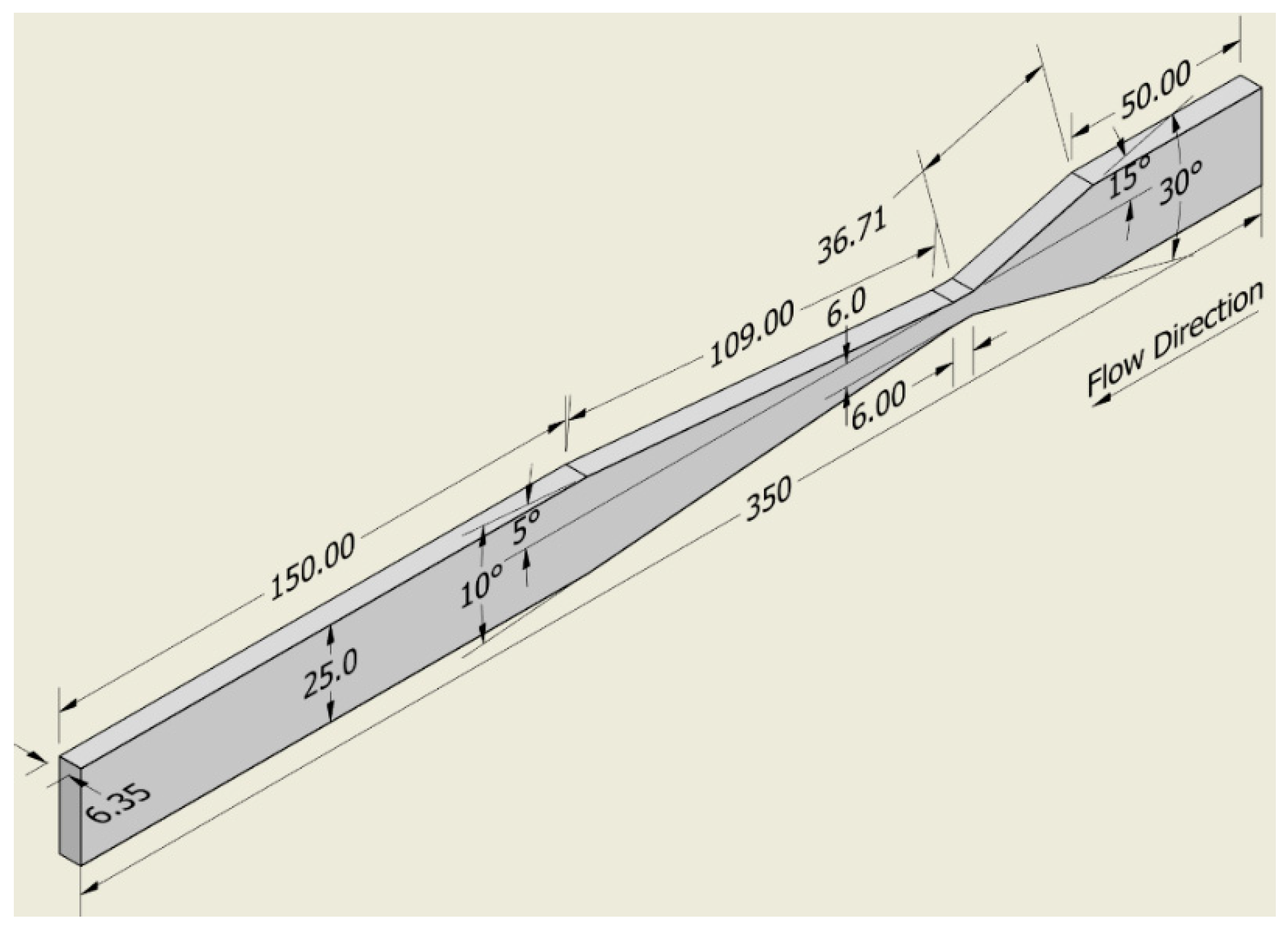
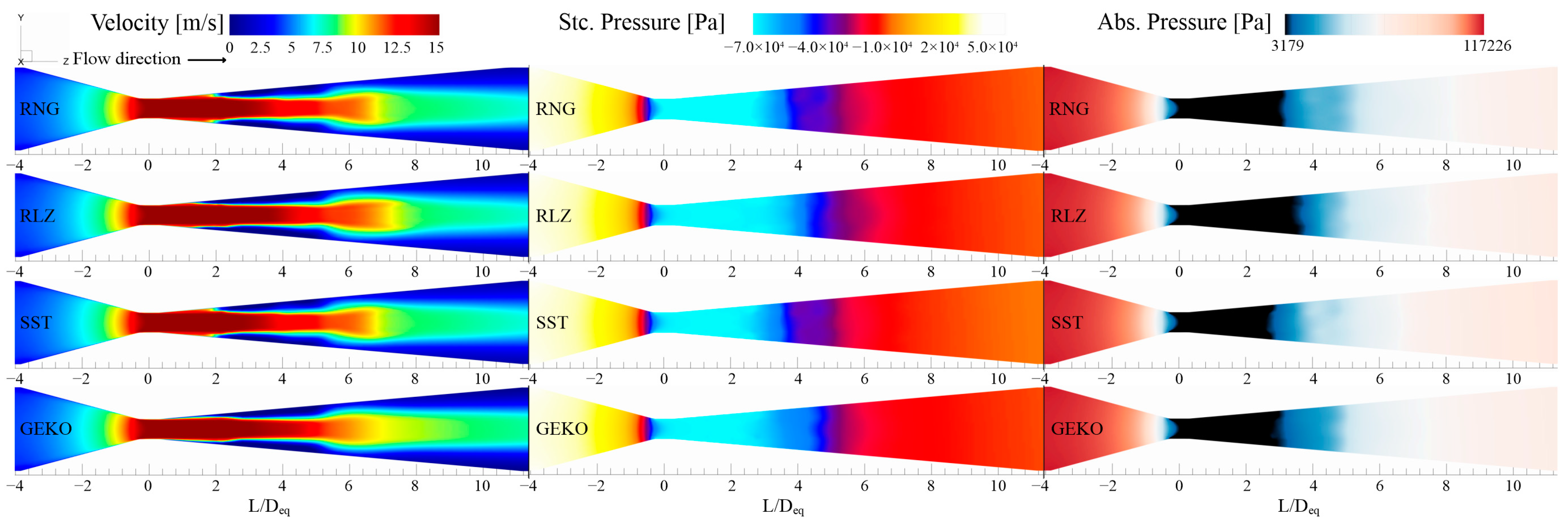
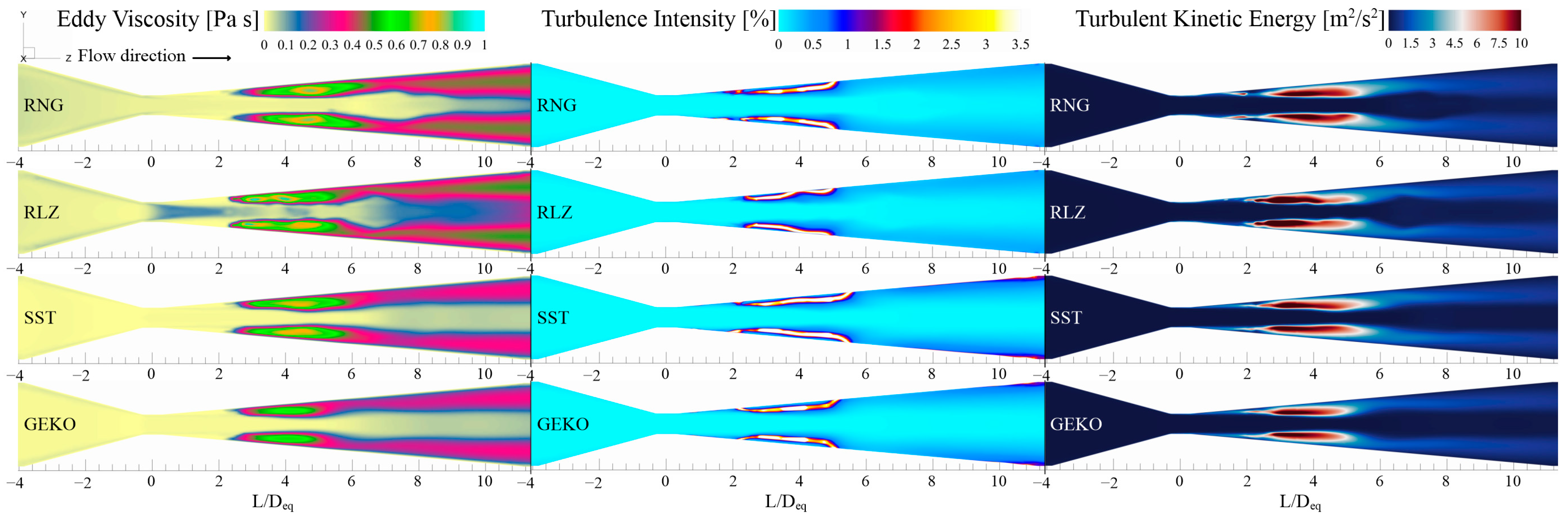
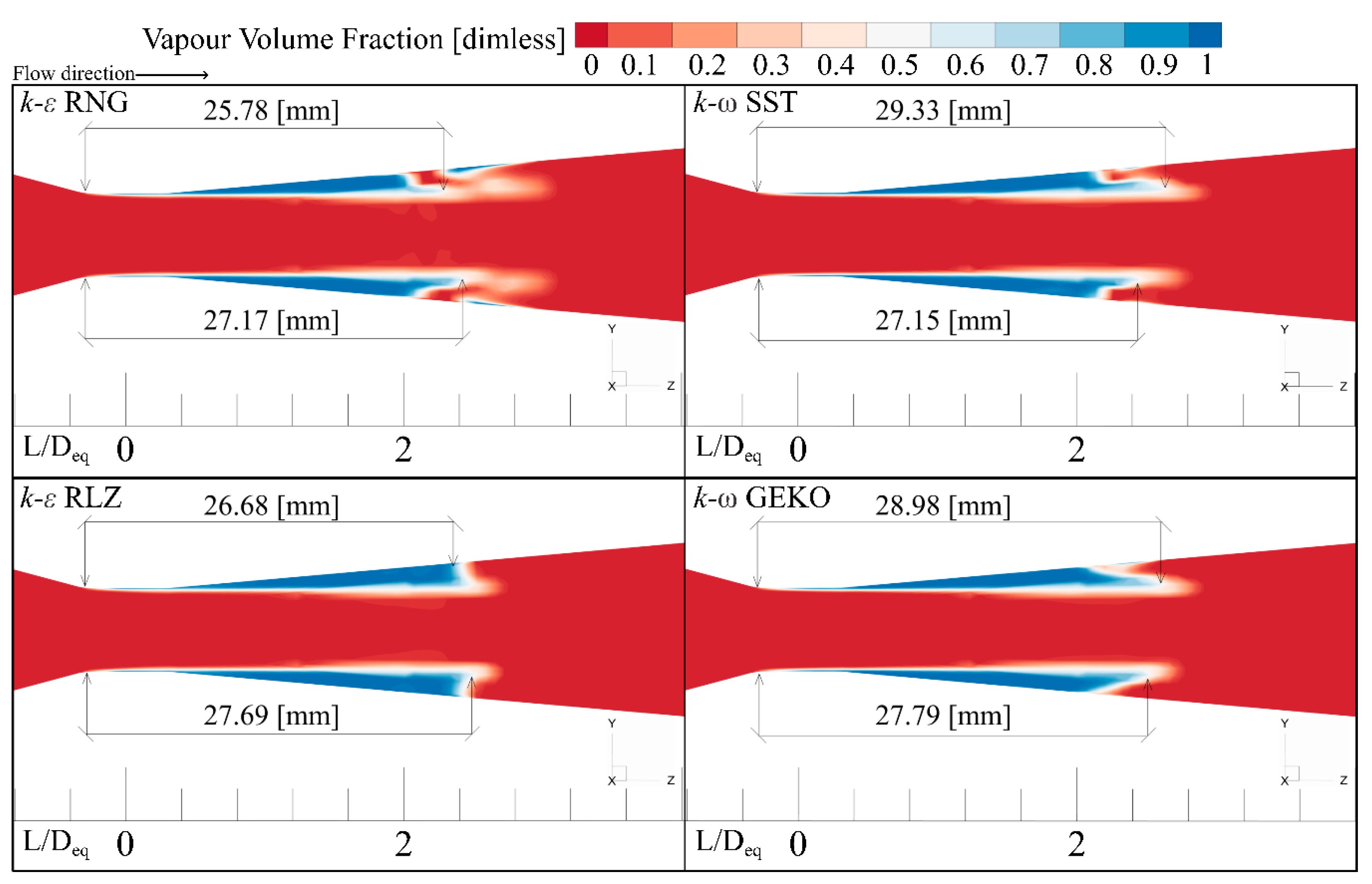
Table 1.
Thermodynamic fluids properties.
| Phase | ||||
|---|---|---|---|---|
| Water liquid | 298.15 | 998.048 | 8.91 × 10⁻⁴ | 0.0725 |
| Water vapor | 0.023 | 9.87 × 10⁻⁶ |
Table 2.
Mesh characteristics.
| Mesh | Number of Cells | Computing Time in Hours. |
|---|---|---|
| 1 | 458,880 | ≈3 |
| 2 | 585,816 | ≈5 |
| 3 | 757,008 | ≈16 |
| 4 | 992,953 | ≈27 |
| 5 | 1,859,552 | ≈68 |
| 6 | 2,860,602 | ≈127 |
| 7 | 3,577,320 | ≈187 |
Table 3.
Velocity, static pressure, absolute pressure values, saturation pressure length, and error percent.
Table 3.
Velocity, static pressure, absolute pressure values, saturation pressure length, and error percent.
| Model | Velocity [m/s] | Error % | [Pa] | Error % | [Pa] | Error % | |
|---|---|---|---|---|---|---|---|
| RNG | 14.57 | 4.145 | −53,496.72 | 4.47 | 50,134.62 | 2.066 | 3.2 |
| RLZ | 15.42 | 10.221 | −63,012.03 | 23.05 | 38,726.00 | 24.352 | 3.8 |
| SST | 15.01 | 7.290 | −61,212.44 | 19.53 | 40,961.49 | 19.985 | 2.8 |
| GEKO | 14.87 | 6.290 | −58,654.57 | 14.54 | 43,595.32 | 14.840 | 3.2 |
| Experimental [37] | 13.99 | −51,207.22 | 51,192.77 | N/A |
Table 4.
Vapor cloud length values.
| Model | Min | Error % | Max | Error % | Deviation % | We | |
|---|---|---|---|---|---|---|---|
| RNG | 25.78 | 0.386 | 27.17 | 4.9845 | 26.475 | 2.299 | 53,014.4 |
| RLZ | 26.68 | 3.091 | 27.69 | 6.993 | 27.185 | 5.042 | 56,720.8 |
| SST | 27.15 | 4.907 | 29.33 | 13.330 | 28.24 | 9.119 | 46,495.9 |
| GEKO | 27.79 | 7.380 | 28.79 | 11.244 | 28.29 | 9.312 | 48,348.9 |
| Experimental [37] | 25.88 | 27 | 26.44 |
Disclaimer/Publisher’s Note: The statements, opinions and data contained in all publications are solely those of the individual author(s) and contributor(s) and not of MDPI and/or the editor(s). MDPI and/or the editor(s) disclaim responsibility for any injury to people or property resulting from any ideas, methods, instructions or products referred to in the content. |
© 2024 by the authors. Licensee MDPI, Basel, Switzerland. This article is an open access article distributed under the terms and conditions of the Creative Commons Attribution (CC BY) license (https://creativecommons.org/licenses/by/4.0/).
Share and Cite
MDPI and ACS Style
De la Cruz-Ávila, M.; De León-Ruiz, J.E.; Carvajal-Mariscal, I.; Klapp, J. CFD Turbulence Models Assessment for the Cavitation Phenomenon in a Rectangular Profile Venturi Tube. Fluids 2024, 9, 71. https://doi.org/10.3390/fluids9030071
AMA Style
De la Cruz-Ávila M, De León-Ruiz JE, Carvajal-Mariscal I, Klapp J. CFD Turbulence Models Assessment for the Cavitation Phenomenon in a Rectangular Profile Venturi Tube. Fluids. 2024; 9(3):71. https://doi.org/10.3390/fluids9030071
Chicago/Turabian StyleDe la Cruz-Ávila, Mauricio, Jorge E. De León-Ruiz, Ignacio Carvajal-Mariscal, and Jaime Klapp. 2024. "CFD Turbulence Models Assessment for the Cavitation Phenomenon in a Rectangular Profile Venturi Tube" Fluids 9, no. 3: 71. https://doi.org/10.3390/fluids9030071